The average value is a generalizing characteristic of a set of similar social phenomena according to one quantitative feature in certain conditions of place and time.
When calculating the average generalizing indicators, the typical dimensions of the level of a particular feature common to this system are revealed and thereby the typical features and properties common to it are revealed.
The method of average values is a special form of statistical generalization. The use of the method of average values is possible only if there is a variation of the feature in a set of homogeneous phenomena.
Average values can be both absolute and relative (average salary, average percentage of plan implementation).
The level of the feature in individual units of the aggregate is formed under the influence of various conditions, some of them are common to all units, others are random. In the average value, calculated on the basis of data on a large number of units, fluctuations in the size of the feature caused by random causes are extinguished, and a common property for the whole population is manifested. When averaging, all deviations of the feature from the average level were balanced, i.e. there was a distraction (abstraction) from the individual characteristics of individual units, i.e. the average value is abstract, and this is its scientific value.
The average value correctly characterizes homogeneous aggregates in their content. Such an average will be typical, since it reflects the general that is characteristic of a given set of social phenomena.
If the totality as a whole is heterogeneous in composition, then in order to obtain typical averages, it is necessary to divide such a set into homogeneous groups using the grouping method and then calculate the average values for each group separately.
The average value is always named, it has the same dimension as the feature of the individual units of the population.
Objectivity and typicality of the statistical average can be ensured only under certain conditions. The first condition is that the mean must be calculated for a qualitatively homogeneous population. The second condition is that not single, but mass data should be used to calculate the average, because only then possible random deviations are mutually extinguished.
It should be remembered that excessive enthusiasm for average indicators can lead to biased conclusions when conducting an analysis. This is due to the fact that average values, being generalizing indicators, extinguish, ignore those differences in the quantitative features of individual units of the population that really exist and may be of independent interest.
In statistics, several types of average values are used:
arithmetic mean; medium harmonic; mean quadratic; geometric mean; average chronological.
These means belong to the class of power averages. In addition to them, structural averages are used – fashion and median.
The arithmetic mean is the main type of means. It can be simple and balanced.
The arithmetic mean of the prime is calculated by dividing the sum of the values of the feature by the number of values:
![]()
![]()
![]() ,
,
where ![]()
![]() is the arithmetic mean;
is the arithmetic mean;
![]()
![]() – individual values of the feature;
– individual values of the feature;
![]()
![]() is the number of feature values.
is the number of feature values.
Example.
As of 14 October, the following data are available on metal consumption by 8 workers (kg): 17.2; 19,0; 20,0; 17,0; 18,0; 19,8; 18,0; 18.6 In order to determine the average consumption of metal per worker, it is necessary to divide the total consumption of metal by the number of workers:
![]()
![]() kg.
kg.
If the data are presented in the form of a discrete series of distribution, then the calculation of the mean is made according to the formula of the arithmetic weighted mean:
 ,
,
where x is the value of the feature;
f is the frequency of repetition of the corresponding trait (weight).
Example.
Table 12 Resource requirements by component
Time spent on part processing
Time (sec) On Machining Part(x) | 46 | 48 | 50 |
Number of parts (f) | 250 | 400 | 150 |
Determine the average time spent on part processing:
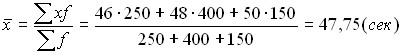 .
.
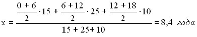
If the data are presented in the form of an interval series of distribution, the principle of calculating the average remains the same, but the average value of the feature for each interval is preliminarily calculated, representing the half-sum of the lower and upper values of the interval:
 ,
,
where: ![]()
![]() ;
;
![]()
![]() – the lower limit of the interval;
– the lower limit of the interval;
![]()
![]() – The upper limit of the interval.
– The upper limit of the interval.
If there are intervals with open boundaries, then for the first group the interval value is taken equal to the interval value of the subsequent group.
Example.
Table 13 Resource requirements by component
Work experience of shop workers
Work experience, years (x) | up to 6 | 6-12 | over 12 |
Number of workers (f) | 15 | 25 | 10 |
Determine the average length of service of shop workers.
It is equal to:
The harmonic mean is the inverse of the arithmetic mean of the inverses. It can be simple and balanced:
simple –  ; weighted – .
The mean quadratic is used when it is necessary to square the variants:
simple –  ; weighted – .
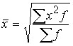
The mean quadratic is used in the technique to calculate the average squared deviation.
Geometric mean – . ![]()
![]()
The average chronological:
simple – ; 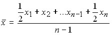
(It is used when the time intervals between phenomena are equal.)
weighted – ; 
(It is used when the time intervals between phenomena are unequal.
Properties of the arithmetic mean.
1. The arithmetic mean of constant numbers is equal to this constant number.
Let x = a, then: 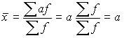 .
.
2. If the weights of all variants are proportionally changed, i.e. increase or decrease by the same number of times, then the arithmetic mean of the new series will not change from this. Let f be reduced by a factor. Then:
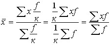 .
.
3. If all the options are reduced or increased by any number, the arithmetic mean of the new series will decrease or increase by the same amount.
Let’s reduce all options x to a, i.e. ![]()
![]() . Then:
. Then:
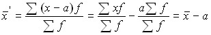 .
.
The arithmetic mean of the original series can be obtained by adding to the arithmetic mean of the new series, the number a previously subtracted from the variants, i.e. ![]()
![]() .
.
4. If all options are reduced by a factor, then the arithmetic mean of the new series will decrease by a factor of one.
Let ![]()
![]() , then
, then 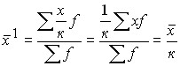 .
.
The arithmetic mean of the original series can be obtained by increasing the arithmetic mean of the ![]()
![]() new series by a factor of :
new series by a factor of : ![]() .
.
5. The sum of the positive and negative deviations of the individual variants from the average, multiplied by weights, is zero.
![]()
![]() .
.
These properties allow, if necessary, to simplify calculations by replacing absolute frequencies with relative ones, to reduce the variants by any number a, to reduce them by a factor and calculate the arithmetic mean of the reduced options, and then proceed to the middle of the original series. The method of calculating the arithmetic mean using its properties is known in statistics as the method of “conditional zero” or “conditional mean”, as well as the “method of moments”.
This method of calculation is reflected in the following formula: 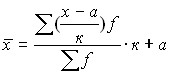 .
.
If the reduced variants  are denoted by
![]() , then
, then ![]() .
.
To characterize the average value of the feature in the variation series, the arithmetic mean, fashion and median are used.
Fashion is the most common meaning of a trait in the aggregate. The median is the numerical value of a feature located in the middle of a ranked series, which divides this series into two equal parts. To determine the median, first find its place in the series by the formula ![]()
![]() , where n is the number of members of the series (
, where n is the number of members of the series (![]() ). If the number of units is even, then the place of the median in the series is defined as
). If the number of units is even, then the place of the median in the series is defined as ![]() .
.
Fashion is used in expert assessments, in determining the size of products that is in the greatest demand (clothes, shoes), the median is used in statistical control of product quality.
Example.
Table 14 Resource requirements by component
Distribution of workshop workers by qualification
tariff category (x) | II | III | IV | V | VI |
number of workers (f) | 10 | 22 | 48 | 55 | 20 |
Accumulated frequencies (F) | 10 | 32 | 80 | 135 | 155 |
The modal is the V digit because it has the highest frequency (![]()
![]() ).
).
The place of the median in the row: ![]()
![]() .
.
The median is iv category. To determine the median, accumulated frequencies were used, which are obtained by sequential summation of frequencies. The accumulated frequency for the II digit is equal to its frequency, for the III digit it is the sum of the frequency of the III discharge and the accumulated frequency of the II digit, that is, 22 + 10 = 32, etc.
When calculating modes and medians in an interval series, you must first determine the interval in which they are located, the average value of this interval corresponds to their approximate value.
Example.
Table 15 Resource requirements by component
Distribution of cars by daily mileage
Daily mileage (x) | 90-130 | 130-160 | 160-190 | 190-230 | 230-270 |
Number of vehicles (f) | 70 | 160 | 130 | 85 | 20 |
Accumulated frequencies (F) | 70 | 230 | 360 | 445 | 465 |
The modal interval is [130 – 160], the average value of which is 145 km; Mo = 145 km.
![]()
![]() From the accumulated frequencies, we determine the median interval [160 – 190] [Me = 175 km].
From the accumulated frequencies, we determine the median interval [160 – 190] [Me = 175 km].
To determine the fashion in series with equal distribution intervals, the modal interval is determined by the highest frequency, and in series with unequal intervals by the highest density of distribution.
To determine the fashion in rows with equal intervals, the formula is used:
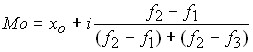 ,
,
where ![]()
![]() is the lower limit of the modal interval;
is the lower limit of the modal interval;
![]()
![]() – the value of the interval;
– the value of the interval;
![]()
![]() – frequencies of the premodal, modal and postmodal intervals.
– frequencies of the premodal, modal and postmodal intervals.
Fashion can be determined graphically by the histogram. To do this, in the highest column of the histogram from the boundaries of 2 adjacent columns, lines are drawn, then from the point of their intersection, perpendicular to the abscissa axis are lowered. The value of the sign is on the abscissa axis and will correspond to the fashion.
To calculate the median in the interval series, we will use the following formulas:
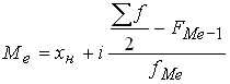 ,
,
or 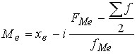 ,
,
Where is:
![]()
![]() – the lower limit of the median interval; i is the value of the median interval;
– the lower limit of the median interval; i is the value of the median interval;
![]()
![]() – Serial number of the median;
– Serial number of the median;
![]()
![]() – frequency accumulated up to the median interval;
– frequency accumulated up to the median interval;
![]()
![]() – The frequency of the median interval.
– The frequency of the median interval.
![]()
![]() – the upper limit of the median interval;
– the upper limit of the median interval;
![]()
![]() – Accumulated median interval frequency.
– Accumulated median interval frequency.
The median can be defined graphically. For this purpose, a cumulative is built. To determine the Me, the height of the largest ordinate is divided in half. Through the resulting point, a straight line parallel to the abscissa axis is drawn until it intersects with the cumulative. The abscissa is the point of intersection and is Me.
Along with the median, for a more complete description of the population, other values of variants are used, occupying a well-defined position in the ranked series. These include quartiles and decili.
Quartiles divide a series according to the sum of frequencies into 4 equal parts, and deciles into 10 equal parts. There are three quartiles and nine deciles.
The calculation of these indicators in the variation series is similar to the calculation of the median. It begins with finding the sequence number of the corresponding variant and determining from the accumulated frequencies the interval in which this variant is located. Formulas for quartiles in the interval variation series are as follows:
lower (or first quartile)
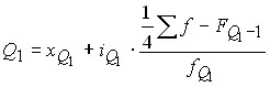 ,
,
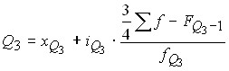
top (or third quartile)
 ,
,
Where is:
![]()
![]() – the lower bounds of the respective quartile intervals;
– the lower bounds of the respective quartile intervals;
![]()
![]() – the value of the corresponding interval;
– the value of the corresponding interval;
![]()
![]() is the sum of the frequencies of the series;
is the sum of the frequencies of the series;
![]()
![]() – the accumulated frequencies of the intervals preceding the corresponding quartile ones;
– the accumulated frequencies of the intervals preceding the corresponding quartile ones;
![]()
![]() – the frequencies corresponding to quartile intervals.
– the frequencies corresponding to quartile intervals.
The second quartile is the median.
The relationship between the arithmetic mean, fashion and median can be judged on the nature of the distribution. In symmetrical distributions, all three indicators coincide. The greater the discrepancy between the mode and the arithmetic mean, the more asymmetrical the series.
It has been empirically established that for moderately asymmetric series, the difference between the mode and the arithmetic mean is about 3 times greater than the difference between the median and the mean ![]()
![]() . This ratio can be used in some cases to determine the third indicator for two known ones.
. This ratio can be used in some cases to determine the third indicator for two known ones.
Security questions
What is called the average in statistics? Methods for determining the arithmetic mean. Basic properties of the arithmetic mean. What is fashion and ways to calculate it. What is the median and how to calculate it.