A variation of a feature is a difference in the numerical values of a trait in individual units of the population. The size of the variation allows us to judge how homogeneous the group under study is and, consequently, how characteristic the average group is. The study of deviations from the average is of great practical and theoretical importance, since the development of the phenomenon is manifested in deviations.
Statistics are presented in the distribution series. Depending on the feature underlying the grouping of data, attribute and variation series are distinguished. The numerical values of a feature that occur in a given population are called variants of values. Statistical data without any systematization form a primary series.
Example.
CHP No | 1 | 2 | 3 | 4 | 5 |
Cost price 1 kWh, thousand rubles. | 5,8 | 6,6 | 5,9 | 6,7 | 6,6 |
If there is a sufficiently large number of variants of the values of the feature, it is necessary to order the primary series to study it, i.e. rank – arrange all variants of the series in an increasing (or decreasing) order.
CHP No | 1 | 2 | 3 | 4 | 5 |
Cost price 1 kWh, thousand rubles. | 5,8 | 5,9 | 6,6 | 6,6 | 6,7 |
When looking at the ranked data, you can see that the variants of the values of the feature in individual units are repeated. The number of repetitions of individual variants is called the repetition rate (![]()
![]() ).
).
By the nature of the variation, discrete and continuous signs are distinguished. Discrete features differ from each other by some discontinuous number.
Table 16 Resource requirements
Distribution of workshop workers by qualification
Tariff Discharge ( | Number of workers | Frequencies (
| Accumulated frequencies (Fi) |
II | 1 | 0,05 | 1 |
III | 5 | 0,25 | 6 |
IV | 8 | 0,40 | 14 |
V | 4 | 0,20 | 18 |
VI | 2 | 0,10 | 20 |
Total: | 20 | 1,00 |
Instead of the absolute number of workers who have a certain rank, you can set the proportion of workers in that rank. Frequencies represented in relative terms are called frequencies and denote ![]()
![]() :
:
 .
.
Frequencies can be expressed in fractions of one or as a percentage. The accumulated frequencies are determined by sequential summation of frequencies.
Continuous features can differ from one another by an arbitrarily small amount and within certain boundaries take any values. To construct a series of distributions of continuous features, the values of the variants are indicated in the intervals “from – to”. When constructing interval series, it is necessary to determine the number of intervals and determine the size of the interval:
![]()
![]() .
.
If the variation series is given in unequal intervals, then the absolute and relative densities of the distribution must be calculated to correctly represent the nature of the distribution. Absolute density:
![]()
![]() ,
,
where ![]()
![]() is the size of the interval.
is the size of the interval.
Relative density:
![]()
![]() ,
,
where ![]()
![]() is the frequency.
is the frequency.
These indicators are used to transform intervals if the data are collected from different populations and processed differently:
![]()
![]() .
.
To characterize the size of the variation, special indicators of oscillation are used: the range of variation, the average linear deviation, the mean quadratic deviation, the coefficient of variation.
The range of variation is the magnitude of the difference between the maximum and minimum values of the feature:
![]()
![]() .
.
The advantage of this indicator is the simplicity of calculation. The disadvantage is that this indicator relies only on two extreme values of the feature and does not take into account the degree of oscillation of the bulk of the members of the series.
The mean linear deviation is the arithmetic mean of the absolute deviations of the individual values of the feature from the average value.
For the primary series: 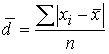 .
.
For the distribution series: 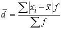 .
.
Since, according to the property of the arithmetic mean, the algebraic sum of the deviations of the individual values of the feature from the arithmetic mean is zero, the absolute values of individual deviations are summed up for the calculation ![]()
![]() , regardless of the sign.
, regardless of the sign.
The mean linear deviation shows how much, on average, the individual values of the feature differ from their average value.
The mean square deviation is equal to the square root of the mean square deviations of the individual values of the feature from the arithmetic mean.
For the primary series: 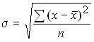 .
.
For the distribution series: 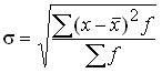 .
.
The mean linear and mean quadratic deviations show how much the value of the feature fluctuates on average in the units of the studied population: ![]()
![]() >
>![]() . For moderately asymmetric distribution series, the following ratio is established:
. For moderately asymmetric distribution series, the following ratio is established: ![]() or
or ![]() .
.
Variance has an independent value in statistics and is one of the most important indicators:
For the primary series: 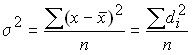 .
.
For the variation series: 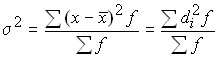 .
.
Hence: ![]()
![]() .
.
In statistics, it is often necessary to compare the variations of various features. In such cases, an indicator of relative scattering is used – the coefficient of variation:
![]()
![]()
![]() .
.
The coefficient of variation shows by what percentage on average the individual values differ from the arithmetic mean. It is a criterion for the reliability of the average: if it exceeds 40%, then this indicates a large oscillation of the feature and, therefore, the average is not reliable enough.
Linear coefficient of variation: 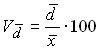 .
.
Oscillation coefficient: ![]()
![]() .
.
Dispersion has a number of properties.
1. The variance of a constant number is zero. If ![]()
![]() then
then ![]()
![]()
![]()
 .
.
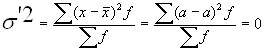
2. If all variants of one series are increased or decreased by any number, the variance of the new series will not change.
Let ![]()
![]() , but then
, but then ![]()
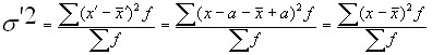 .
.
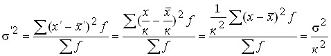
3. If all variants of the series are reduced or increased by ![]()
![]() a factor, then the variance of the new series will decrease (or increase) in
a factor, then the variance of the new series will decrease (or increase) in ![]() .
.
Let ![]()
![]() , then
, then ![]()
![]()
![]()
 .
.
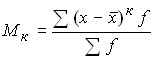
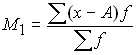
The moment of distribution is called the arithmetic mean of certain degrees of deviations of individual values of the feature from a certain initial value. In general, the moment can be written as follows:
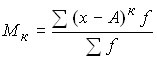 ,
,
where A is the value from which the deviations are determined;
k is the degree of deviation (order of moment).
Depending on the value, the moments can be calculated of any order, but the moments of the first four orders are practically used.
Any number can be taken as a constant value A. Depending on what is taken as a constant value, the following three types of moments are distinguished:
1) if zero is taken as a constant value, i.e. A = 0, then the moments are called initial. In general, they can be written:
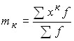 and, accordingly, the moments of the first four orders;
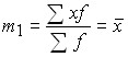 ;
;
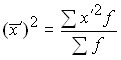
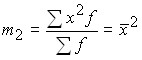 – the arithmetic mean of the squares of the variants;
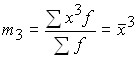 ;
;
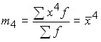 .
.
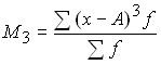
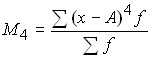
2) if the arithmetic mean series is taken as a constant value, i.e. A = ![]()
![]() , then the moments are called central:
, then the moments are called central:
 ;
;
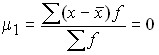 according to the property of the arithmetic mean;
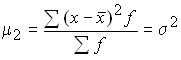 dispersion;
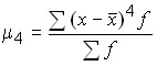 to calculate the excess rate.
3) if any number other than zero is taken as a constant value, then the moment is called conditional:
 ;
;
 ;
;
 ;
;
 ;
;
 .
.
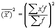
Using the initial moments of the first and second order, it is possible to obtain a formula for calculating the variance:
![]()
![]()
You can also calculate the variance as follows:
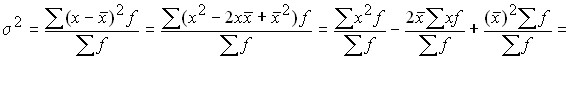
![]()
![]()
Therefore, the variance can be defined as the difference between the average square of the variants and the square of their mean.
In variation series with equal intervals, the variance can be calculated by the method of moments and by the method of reference from the conditional zero.
The calculation is made according to the formula:
![]()
![]() ,
,
Where is:
![]()
![]() – interval width;
– interval width;
![]()
![]() , x0 is a conditional zero, which is convenient to use the middle of the interval with the highest frequency;
, x0 is a conditional zero, which is convenient to use the middle of the interval with the highest frequency;
 – Second-order moment;
 is the square of the first-order moment.
The units of the phenomena under study can be characterized by such features that some units of the aggregate possess, while others do not. Such a sign is called an alternative one.
The presence of a feature is indicated by one, and its absence by zero. The proportion of units possessing this feature is denoted by p, and the fraction that does not possess it is q. Therefore, p + q = 1, q = 1 – p. The average value of the alternative feature is:
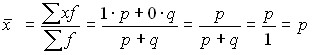 .
.
Thus, the average value of an alternative feature is equal to the value of the fraction of units that possess it.
Let’s determine the variance:
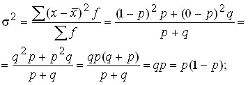
![]()
![]() .
.
Example.
Of the 1,000 finished products, 250 were of the highest quality. Define ![]()
![]() .
.
![]()
![]() or 25% of the highest quality products.
or 25% of the highest quality products.
![]()
![]()
![]()
![]() .
.
To assess the influence of various factors that determine the oscillation of individual values of the trait, it is possible to use the decomposition of variance into components: intergroup and intragroup variance.
The variation due to the influence of the factor underlying the grouping is characterized by intergroup variance, which is a measure of the oscillation of particular averages by groups from the total average:
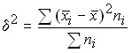 ,
,
where ![]()
![]() are the group averages,
are the group averages,
![]()
![]() – the total average for the whole population,
– the total average for the whole population,
![]()
![]() – Number of individual groups.
– Number of individual groups.
Variation due to the influence of other factors is characterized in each group by group variance:
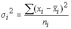 ,
,
and for the population as a whole, the average of the intragroup variances:
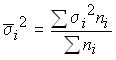 .
.
Therefore, the total variation of the trait in the aggregate should be defined as the sum of the variation of the group averages (due to one isolated factor) and the residual variation (due to other factors). This equality is reflected in the rule of addition of variances ![]()
![]() .
.
The ratio of intergroup variance ![]()
![]() to the total
to the total ![]() is given by the coefficient of
is given by the coefficient of  determination , which characterizes the proportion of variation of the resulting feature due to the variation of the factor feature (which is the basis of the grouping).
The coefficient of empirical correlation characterizes 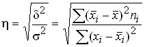 the closeness of the relationship between the effective and factor features.
To get an idea of the form of distribution, distribution graphs (polygon and histogram) are built. The number of observations from which the empirical distribution is constructed is usually small and is a sample from the general population under study. With an increase in the number of observations and at the same time a decrease in the size of the interval, the zigzags of the polygon begin to smooth out, and in the limit we come to a smooth curve, which is called the distribution curve.
Statistics investigate different types of distribution. As a rule, they are single-vertex. Polyversity indicates the heterogeneity of the population under study. The appearance of two or more vertices indicates the need to rearrange the data in order to highlight more homogeneous groups.
A symmetric distribution is one in which the frequencies of any two variants equal in both directions from the center of distribution are equal to each other. For symmetric distributions, the arithmetic mean, the mode, and the median are equal. The simplest indicator of asymmetry is based on the ratio of indicators of the center of distribution: the greater the difference between the arithmetic mean and the mode (median), the greater the asymmetry of the series.
Asymmetry index:
![]()
![]() or
or ![]() .
.
To compare asymmetry in several rows, a relative asymmetry indicator is used.
![]()
![]() or .
or . ![]()
![]()
![]() The value can be positive and negative. If
The value can be positive and negative. If ![]() , then on the graph such a series will have an elongation to the right (right-sided asymmetry), if
, then on the graph such a series will have an elongation to the right (right-sided asymmetry), if ![]() , then an elongation to the left (left-sided asymmetry).
, then an elongation to the left (left-sided asymmetry).
The steepness characteristic of the distribution is also calculated. This is an indicator of excess. With the same arithmetic mean, the empirical series may be peaked or low-vertex compared to the normal distribution curve. The excess rate reflects this feature:
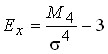 .
.
If ![]()
![]() the > 0, then the excess is considered positive (the distribution is peaked), if
the > 0, then the excess is considered positive (the distribution is peaked), if ![]() the < 0, then the excess is considered negative (the distribution is low-vertex).
the < 0, then the excess is considered negative (the distribution is low-vertex).
Among the various distribution curves, a special place is occupied by the normal distribution. The normal distribution in a graph is a symmetrical bell curve having a maximum at a point ![]()
![]() . This point is the mode and median. The inflection point of a normal curve is ±
. This point is the mode and median. The inflection point of a normal curve is ±![]() away from
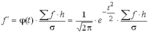
away from ![]() . The normal distribution curve is expressed by Laplace’s equation:
. The normal distribution curve is expressed by Laplace’s equation:
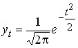 ,
,
where t is the normalized deviation, . ![]()
![]()
It is established that if the area bounded by the normal distribution curve is taken as 100%, then it is possible to calculate the area enclosed between the curve and any two ordinates. It is established that the area between ordinates drawn at a distance ![]()
![]() on each side of
on each side of ![]() , is 0.683 of the total area. This means that 68.3% of all frequencies (units) deviate from
, is 0.683 of the total area. This means that 68.3% of all frequencies (units) deviate from ![]() no more than
no more than ![]() by , i.e. are within
by , i.e. are within ![]() . the area enclosed between ordinates drawn at a distance of 2
. the area enclosed between ordinates drawn at a distance of 2![]() from
from ![]() in both directions is 0.954, i.e. 95.4% of
in both directions is 0.954, i.e. 95.4% of ![]() all units of the aggregate are within . 99.7% of all units are within . 99.7% of
all units of the aggregate are within . 99.7% of all units are within . 99.7% of ![]() all units are within . . This is the rule of three sigmas, characteristic of the normal distribution.
all units are within . . This is the rule of three sigmas, characteristic of the normal distribution.
Normal distribution is characteristic of phenomena in biology and engineering. In economics, moderately asymmetric distributions are more common.
When dealing with empirical distributions, it can be assumed that each empirical distribution corresponds to a certain, characteristic theoretical curve. Knowledge of the shape of the theoretical curve can be used in various calculations and forecasts. To do this, you need to determine:
the general nature of the distribution; to construct a theoretical curve from empirical data; determine how close the empirical frequencies are to the theoretical ones.
Let’s introduce the designations:
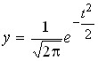 ,
,  ,
,
where ![]()
![]() = 2.7182 (base of the natural logarithm);
= 2.7182 (base of the natural logarithm);
![]()
![]() = 3,14.
= 3,14.
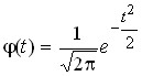
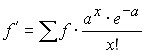
To construct a theoretical curve of normal distribution from empirical data, it is necessary to find theoretical frequencies:
 ,
,
where  is a constant;
h is the width of the interval;
![]()
![]() is the tabulated value that is located by deviations t.
is the tabulated value that is located by deviations t.
The sequence of calculation of theoretical frequencies is as follows:
the arithmetic mean of the series![]()
![]() is calculated; the mean quadratic deviation
is calculated; the mean quadratic deviation ![]() is calculated; is located
is calculated; is located ![]() ; according to the found t on the table is
; according to the found t on the table is ![]() ; calculated
; calculated ![]() ; each value
; each value ![]() is multiplied by
is multiplied by  .
.
Among the most important theoretical distributions is the Poisson distribution, which is characteristic of rare phenomena, and with an increase in the value of x, the probability of their occurrence decreases.
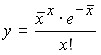
The Poisson distribution is as follows:
 ,
,
where ![]()
![]() .
.
Then:
 .
.
Graphically, it looks like this:
Finding the theoretical frequencies when aligning a series with the Poisson distribution is done in the following order:
is the arithmetic mean, ![]()
![]() ; the table determines
; the table determines ![]() ; for each value x the theoretical frequency is determined.
; for each value x the theoretical frequency is determined.
A number of criteria are used in statistics to assess the randomness or materiality of discrepancies between the frequencies of empirical and theoretical distributions.
One of the main criteria for comparing the frequencies of empirical and theoretical distributions is the Pearson consensus criterion (![]()
![]() – square):
– square):
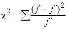 ,
,
where ![]()
![]() are the empirical frequencies;
are the empirical frequencies;
![]()
![]() – theoretical frequencies.
– theoretical frequencies.
To assess the proximity of the empirical distribution to the theoretical one, the probability ![]()
![]() of this criterion reaching this value is determined. If
of this criterion reaching this value is determined. If ![]() the > 0.05, then the deviations of the actual frequencies from the theoretical ones are considered random, insignificant. If
the > 0.05, then the deviations of the actual frequencies from the theoretical ones are considered random, insignificant. If ![]() <0.05, then the deviations are significant, and the empirical distribution is fundamentally different from the theoretical one. The values of the tabulation probabilities
<0.05, then the deviations are significant, and the empirical distribution is fundamentally different from the theoretical one. The values of the tabulation probabilities ![]() depending on and the
depending on and the ![]() number of degrees of freedom
number of degrees of freedom ![]() . For the normal distribution
. For the normal distribution ![]() , for the Poisson curve distribution:
, for the Poisson curve distribution: ![]() . Knowing the
. Knowing the ![]() calculated , we compare it with the tabular (limit). If
calculated , we compare it with the tabular (limit). If ![]() the actual > tabular, then the
the actual > tabular, then the ![]() discrepancy between the frequencies of the empirical and theoretical distributions cannot be considered random. If
discrepancy between the frequencies of the empirical and theoretical distributions cannot be considered random. If ![]() the actual <
the actual < ![]() tabular, then the discrepancy can be considered random, and the theoretical distribution in question is suitable for describing the empirical distribution.
tabular, then the discrepancy can be considered random, and the theoretical distribution in question is suitable for describing the empirical distribution.
Romanovsky’s criterion is defined by:
 ,
,
where ![]()
![]() is the Pearson criterion;
is the Pearson criterion;
k is the number of units of degrees of freedom.
If this criterion , then the ![]()
![]() discrepancies cannot be considered random. If it < 3, then the discrepancy between the empirical and theoretical frequencies can be considered random.
discrepancies cannot be considered random. If it < 3, then the discrepancy between the empirical and theoretical frequencies can be considered random.
A.N. Kolmogorov proposed a criterion based on a comparison of the distribution of the accumulation of accumulated frequencies (frequencies):
![]()
![]() ,
,
where d is the maximum difference between the accumulated rates of the empirical and theoretical distribution series, and N is the number of units of the population. If the distribution is given in frequencies, then:
![]()
![]() ,
,
where D is the maximum difference between the accumulated frequencies of the two distributions.