The development of the model of “groping” the equilibrium state is a model of the functioning of the market, built on the basis of an iterative method for solving convex programming problems, the essence of which is as follows: the problem of maximizing the upward convex functions of n-variables is considered.
![]()
![]()
under the conditions of:
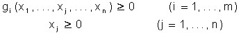 ,
,
where the functions ![]()
![]() are also convex.
are also convex.
The non-negative saddle point of the Lagrange function is:
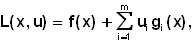
where ui are Lagrange multipliers (dual variables), called the point (![]()
![]() ) for which the relations are executed
) for which the relations are executed
![]()
![]()
for all ![]()
![]() .
.
The following theorem (Kuhn-Tucker) is valid.
If:
1) ![]()
![]() convex functions in
convex functions in ![]() ;
;
2) there is a vector ![]()
![]() such that
such that ![]() , then the vector
, then the vector ![]() will be the optimal solution of the maximization problem formulated above if and only if there exists such a vector
will be the optimal solution of the maximization problem formulated above if and only if there exists such a vector ![]() that (
that (![]() ) is a non-negative saddle point of the Lagrange function L(x,u).
) is a non-negative saddle point of the Lagrange function L(x,u).
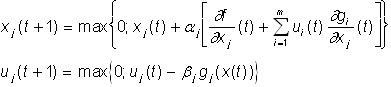
Thus, the solution of the maximization problem is reduced to finding the Lagrange saddle point, which in turn is carried out by applying the following iterative process (C. Arrow, L. Hurwitz):
 .
.
Here t is the iteration number.
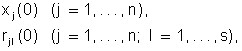
Initial values ![]()
![]() are assumed by known (given) numbers. The presence of the max sign ensures that variables are not negative during the implementation of the iteration process.
are assumed by known (given) numbers. The presence of the max sign ensures that variables are not negative during the implementation of the iteration process.
Positive values ![]()
![]() are called tuning parameters and must be selected small enough to ensure the stability of the process. Various rules are applied to fix the moment when the iteration process ends. As the main ones, it is used as a criterion for the coincidence of the species:
are called tuning parameters and must be selected small enough to ensure the stability of the process. Various rules are applied to fix the moment when the iteration process ends. As the main ones, it is used as a criterion for the coincidence of the species:
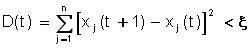 ,
,
where ![]()
![]() is a fairly small number, and setting a certain number (T) of iterations, and then the resulting values:
is a fairly small number, and setting a certain number (T) of iterations, and then the resulting values:
![]()
![]()
are considered to be the coordinates of the saddle point sought. In this case, the vector ![]()
![]() is the solution of the maximization problem, and the vector
is the solution of the maximization problem, and the vector ![]() characterizes the comparative importance of the limitations of the optimization problem.
characterizes the comparative importance of the limitations of the optimization problem.
Consider a complex economic system consisting of the consumer sector, the manufacturing sector, and the resource sector.
Let the consumer sector be represented by a single utility function:
![]()
![]()
where ![]()
![]() is the set of consumable goods that he seeks to maximize.
is the set of consumable goods that he seeks to maximize.
The manufacturing sector consists of n enterprises (productions) (j = 1, …, n) each of them produces one product (in quantity ![]()
![]() ) and they all produce different products. The level of production is determined by the production function
) and they all produce different products. The level of production is determined by the production function
![]()
![]()
where ![]()
![]() are the volumes of production resources used.
are the volumes of production resources used.
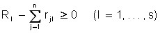
The resource sector is defined by the volume of resources (labor, capital, land, energy, etc.) rl (l = 1, …, s) intended for use in the manufacturing sector. In this case, there are ratios:

The state of equilibrium in the broad sense in the system under consideration is defined as the following ratio between demand (xj) and supply (yj) for all kinds of goods:
![]()
![]()
In the future, we will assume that the utility function U(x) and all production functions ![]()
![]() are convex. In this case, the problem of finding the equilibrium state can be formulated as a convex programming problem:
are convex. In this case, the problem of finding the equilibrium state can be formulated as a convex programming problem:
To find:
![]()
![]()
under the conditions of:
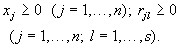
1)![]()
![]() where
where ![]()
2)  ;
;
3) 
As shown above, the solution to this problem in turn boils down to finding the non-negative saddle point of the Lagrange function:
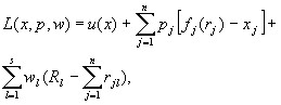
where;
![]()
![]() is the vector of Lagrange multipliers corresponding to the production constraints (1). These values make sense of the prices of different types of products;
is the vector of Lagrange multipliers corresponding to the production constraints (1). These values make sense of the prices of different types of products;
![]()
![]() – the vector of Lagrange multipliers associated with resource constraints (2). The components of this vector are estimates of the importance of factors used in production. For example, the wage rate acts as an estimate of labor resources; the cost of capital services is expressed by an estimate of capital resources, etc.
– the vector of Lagrange multipliers associated with resource constraints (2). The components of this vector are estimates of the importance of factors used in production. For example, the wage rate acts as an estimate of labor resources; the cost of capital services is expressed by an estimate of capital resources, etc.
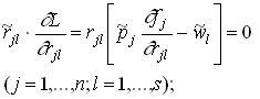
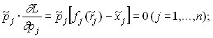
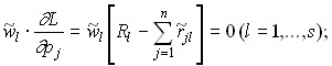
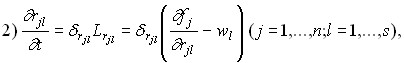
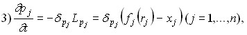
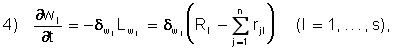
The first-order conditions for finding the saddle point (Kuhn-Tucker conditions) are:
1) 
2) 
3) 
4) 
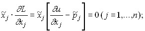
The conditions of the first group have the following economic meaning: if the equilibrium volume of any good (![]()
![]() ) is different from zero, then equality must be met:
) is different from zero, then equality must be met:

which coincides with the condition of the maximum utility function of the consumer in conditions of limited income (see Chapter 1.). Thus, these conditions are the expression of optimal consumer behavior. Note that it follows from the maximal requirement of the Lagrangian function on variables ![]()
![]() that when
that when ![]() :
:

that is, the marginal utility of an unused good does not exceed its price in a state of equilibrium.
The conditions of the second group are that in the case of ![]()
![]() , i.e. in the case when the j-th enterprise uses a non-zero volume of the l-th resource, the ratio must be satisfied:
, i.e. in the case when the j-th enterprise uses a non-zero volume of the l-th resource, the ratio must be satisfied:
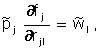
which can be interpreted as a necessary condition for the maximum profit of the enterprise (see Chapter 4). This means that in a state of equilibrium, an optimal production program is carried out for all enterprises.
If the l-th resource is not consumed on the j-volume of the enterprise, i.e. ![]()
![]() , then from the maximization of the Lagrange function we
, then from the maximization of the Lagrange function we ![]() have:
have:

i.e. the marginal productivity of this resource at the j-th enterprise is not higher than its price (the resource is too expensive and relatively inefficient).
The conditions of the third group characterize the relationship between supply and demand of any good in a state of equilibrium. If the price is a ![]()
![]() good, then it is necessary:
good, then it is necessary:
![]()
![]()
i.e. there is an equality of supply and demand![]()
![]() (
(![]() ) of this good. If the equilibrium price
) of this good. If the equilibrium price ![]() is , then it follows from the requirement of the minimum of the Lagrangian
is , then it follows from the requirement of the minimum of the Lagrangian ![]() function that:
function that:
![]()
![]()
i.e. the supply of a good (as a rule) exceeds the demand for it.
The conditions of the fourth group are related to the distribution of resources between enterprises and the assessment of the importance of these resources. If the equilibrium price of the l-th resource ![]()
![]() , then there is an equality:
, then there is an equality:

which indicates the full use of the resource reserve (the demand for the resource is equal to its supply). If , then from the ![]()
![]() condition of minimality of the Lagrange function by variable
condition of minimality of the Lagrange function by variable ![]() follows: i.e. the supply of a resource is not less than the demand for it.
follows: i.e. the supply of a resource is not less than the demand for it.
The procedure for finding a non-negative saddle point is implemented by specifying the general iterative process presented above. Initial values of phase variables:
 ,
,
and dual variables (prices)
![]()
![]()
are considered famous. The following values are determined by the formulas:
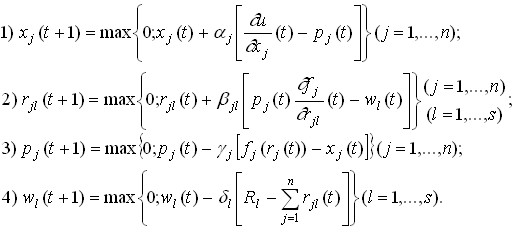
Here, the positive numbers ![]()
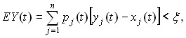
![]() are the settings. As a sign of the end of the calculations, either a fixed number of iterations (T) is usually used, or the iterative process stops and the equilibrium state is considered found if the condition is met:
are the settings. As a sign of the end of the calculations, either a fixed number of iterations (T) is usually used, or the iterative process stops and the equilibrium state is considered found if the condition is met:
where ![]()
![]() is the specified number;
is the specified number;
![]()
![]()
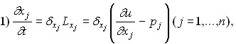
It is also useful to give analogues of iterative formulas in differential form:
Where is 
where 
where ![]()
![]()
where ![]()
![]()
Analysis of this iterative process shows that it quite accurately simulates the market mechanism for achieving a state of equilibrium by changing the volume of demand for goods and resources, as well as by varying the corresponding prices. As can be seen, the consumer’s demand for some good increases as long as its marginal utility exceeds the price of that good, which in turn increases if the demand is greater than the supply of the good from the productive sector. In the same way, the demand of production for resources is regulated: it increases until the marginal efficiency of the resource is greater than its price, i.e. the enterprise has an additional profit from the acquisition of the resource, and growth stops when this profit becomes zero. The price of a resource also increases if the demand for it exceeds the supply from the resource sector, and when equality of supply and demand is achieved, the price becomes unchanged.