Spider-like model of market price dynamics. Assumptions and main components of the model
All the theoretical constructions presented in this work are based on the assumption that the perfect nature of competition is that all households and enterprises act in accordance with market prices. In other words, we are talking about a parametric pricing system.
The main problems faced in accepting such a premise are the following: how the equilibrium of supply and demand is achieved in a market with perfect competition, how market prices are set, how the volume of trade operations is determined – the number of transactions. This topic – the study of the process of market regulation is devoted to this section.
In the graphic image, the process of market regulation is represented in the form of a model, which is called spider-like. When considering, it is important to introduce some assumptions. For this model, it is required to build a supply function, assuming that there is one product and only its price can change, and all other factors on which the demand for this product depends (prices for other goods, basic production assets, the nature of the technology used, taxes and subsidies, natural and climatic conditions) remain unchanged. Therefore, the supply will depend on the volume of the goods (Q) and the price (P): Q = S (p).
The peculiarity of this offer function is that for many types of goods it increases monotonously (S'(p)>0). The growth of supply with an increase in price can be explained by the fact that the optimal volume of output of goods increases, as well as by the fact that new enterprises are included in the industry to produce a highly profitable product. In this case, the supply curve is a geometric place of points – the minimums of the lines of constant profit (line S in Figure 7.16).
The next function used is the demand function, which has the form: Q = D (p).
In the case when the consumer demands a certain product, based on his preferences and budget constraints, if only the price of the goods can change, and all other factors on which the demand for it depends (prices of other goods, monetary income, accumulated savings, etc.) remain unchanged. A characteristic feature of this function is its monotonous decrease for many types of goods, while its graph is a geometric place of points at which the price takes the maximum possible value on the lines of constant utility.
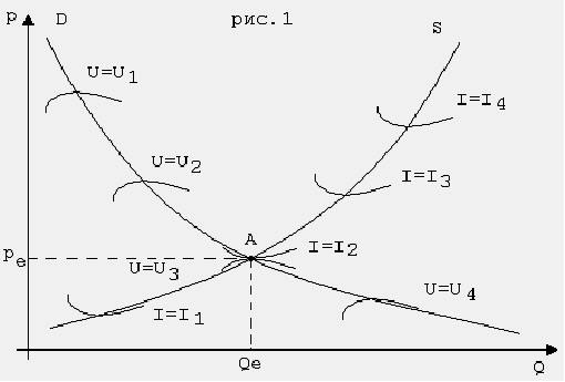
Fig.7.16. Graphs of supply and demand functions
The functions of supply and demand are the main components of the model of the goods market, since they are – according to the assumption – solutions to optimization problems that arise before the participants – buyers and producers.
The intersection of the supply and demand charts occurs at the equilibrium point (point A in Figure 7.16),” and the price Pe corresponding to this point is called equilibrium. If the price in the market is higher than the equilibrium price, then the supply exceeds the demand and overstocking occurs. In this situation, commodity producers (sellers) of many types of goods are ready to reduce the price in order to attract more buyers (for example, if we are talking about perishable goods). Consequently, when the price values are above the equilibrium price, there is a downward pressure on it.
If the price in the market is below equilibrium, then demand exceeds supply, and the product becomes scarce. In this situation, some buyers are ready to pay a higher price for the goods, but reduce the risk and purchase the goods with confidence (for example, if a queue of buyers is formed, then those standing at its end may not receive the goods). Thus, when the price values are below the equilibrium price, there is pressure on it upwards. These two trends lead to the fact that in the markets of many types of goods, as a rule, an equilibrium is established in which demand is equal to supply.
Due to the properties of supply and demand curves, the equilibrium solution is stable in the sense that if the price is strictly fixed and equal to the equilibrium one, then the commodity producer, maximizing profits, supplies the commodity to the market in the amount of S(pe) = Qe; at the same time, the consumer, in an effort to maximize utility, demands D(pe)=Qe. When perfect equilibrium price competition is established in the market, the volume of goods offered by the commodity producer and delivering him the maximum profit at this price is exactly equal to the demand of the consumer.
Dynamic non-equilibrium market models are used to analyze the change in variables (price, demand, supply) over time in the case when the price at the initial moment differs from the equilibrium one. In this case, the process of establishing an equilibrium price can be described by different models using the same functions of supply and demand.
So, variables for a period of time (t,t+1) are taken unchanged. Consequently, successive time intervals (t,t+1) correspond to the values of the price of Pt, demand Dt and supply St. Depending on the hypotheses used in the discrete model of price dynamics, there is either a delay in supply – in this case, we come to the process:
S(P t+1 ) = D(Pt),
or a delay in demand – in this case, we get the process:
D(Pt+1) = S(Pt ).
In both cases, the corresponding iterative process is depicted in the form of a web, which is “wound” on the curves of supply and demand. This provided the basis for a common name for discrete dynamic models.
Discrete demand-lagged models are of greater interest because they reflect decision-making procedures more consistently than continuous ones.