Spider web-like  model with delayed demand

The conceptual model of any process of price dynamics includes the interaction of three subsystems, which can be conditionally called “commodity producer”, “consumer” and “market” (Fig.7.17.). The spider-like model (model A), in which demand lags behind supply by one period: D(Pt+1)=S(Pt), also fits into the scheme of Figure 7.17.

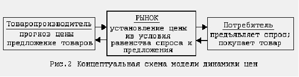
Rice. 7.17. Conceptual scheme of the model of price dynamics

This model is one of the historically first dynamic models of the market, reflecting the behavior of participants. It serves as a good illustration of the application of the modeling method in the analysis of economic processes.

The importance of model A is also determined by the fact that many modern models of price dynamics, as well as dynamic models of macroeconomics, lead to a “spider web-like” process. Consider the hypotheses that underlie this model.

Hypothesis 1. The commodity producer, making a decision on the volume of supply, is guided by the price of the previous period.

This hypothesis means that the commodity producer predicts the price of the next period. True, the forecast here is very primitive, based on a logical scheme: “today the price was Pt, if tomorrow it is equal to Pt, then I will get the maximum benefit when selling the goods in the amount of S (Pt)”.

Hypothesis 2. The market is always in a state of local equilibrium.

This hypothesis can be interpreted, according to Walras, as follows. Instead of the abstract, inanimate concept of “market”, the latter appears in the form of a certain auctioneer who manages the real market. This auctioneer first sets arbitrary prices for goods, after which market participants make conditional transactions and report their result to the auctioneer. If the demand for a certain product turned out to be more (less) than the supply, then the auctioneer changes the initial prices, raising (lowering) the price of this product. Final transactions are made only after equilibrium is reached.

Another interpretation of this hypothesis is that the task of the auctioneer is to establish a maximum price at which all the goods supplied to the market by the manufacturer find a buyer. Formally, these two hypotheses mean the following:

1) the volume of supply on the St+1 market in each period of time t+1 is determined by the value of the price of the previous period using the offer function St+1 = S(Pt);

2) in the market, an equilibrium price of Pt+1 is set in each period t+1, and this price is a solution to the equation D(Pt+1)=St+1;

3) the consumer presents demand, which at the price of Pt + 1 at any given time is equal to the supply of St + 1, as a result of which the consumer acquires everything that is offered to him.

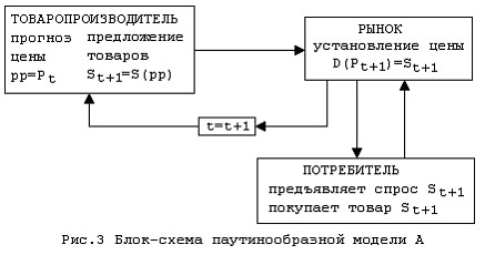
Rice. 7.18. Block diagram of spider web model A

The use of monotonous functions of supply and demand allows you to build a sequence of prices Pt, where t is the step number in time. Indeed, by virtue of hypothesis (1), the producer determines S2 by the value of the price P1 using the supply curve; by virtue of hypothesis (2), the market sets the price of P2 (located using the demand curve); all goods in the amount of S2 find the consumer; by virtue of hypothesis (1), the commodity producer, focusing on the price P2, determines the volume of supply S3, etc. (Fig.7.18.). Next, the process is repeated.

P 

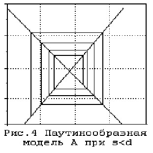
Rice. 7.19. Spider-like model A at s<d

Thus, the formulated hypotheses lead to an iterative process, where demand lags behind supply by one period.

The dynamics of the price (as well as supply and demand) within the framework of this model can be depicted in the form of a curve, which is called either a web or a spiral (Fig. 7.19.). Therefore, in the literature, the spider-like model is sometimes called a “dynamic spiral”. In the case depicted in Figure 7.19., the price sequence Pt tends to the equilibrium level pe, and thus an equilibrium is established here over time.

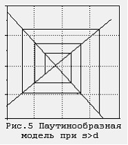
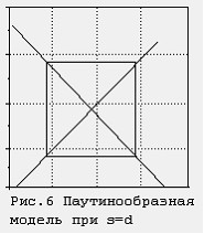
Rice. 7.20. Spider-like model  Fig. 7.21. Spider-like model
  s>d                                                         s=d

At s>d, the amplitude of price fluctuations increases (Figure 7.20.).

At s =d, values equal in absolute value are taken sequentially (Fig.7.21.).

Spider web-like model with delayed supply

Let’s formulate hypotheses of a spider-like model with a delay in supply (model B).

Hypothesis 1. When determining the volume of supply in each period of time, the commodity producer is guided by the demand in the previous period.

This hypothesis leads to an increase (decrease) in supply in the case when demand is greater (less) than supply.

Hypothesis 2. The price of the offered goods is set by the producer at a level determined in accordance with the supply function.

Here, the commodity producer acts formally: he knows that the supply curve is in some sense optimal. Therefore, he believes that when determining the price level using the supply function, the proposed volume of goods will be optimal.

Hypothesis 3. The volume of consumption cannot exceed either the volume of supply or the volume of demand.

This hypothesis means that if supply is less than demand, then consumption is equal to supply.

If demand is less than supply (i.e. there is an oversupply of goods), then consumption is equal to demand, and unsold goods lead to overstocking. Thus, in this model, the relationship between consumption C, demand D, and supply S at each time period t can be represented as:

C = min (S,D).

The latter means that the graph of the consumption curve of model B is the SAD line (Figure 7.22).

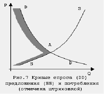
Fig.7.22. Demand curves (DD), supply (SS) and consumption curves (dashed)

The model can be represented in the form of a flowchart shown in Figure 7.23. From this flowchart it can be seen that in this model there is a lag in the supply: S(Pt+1)=D(Pt).

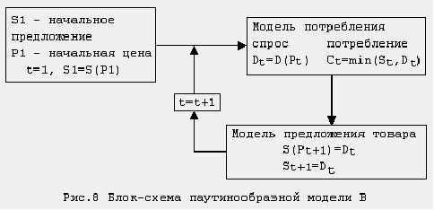
We emphasize that the hypothesis (1), expressing the reaction of the producer to the discrepancy between demand D and supply S, and hypothesis (2) determine the model of supply of goods.

Thinking formally, we come to the following. Given S1 and P1 satisfying the condition S1 = S (P1), the demand for D1 is determined, after which we get C1 = min (S1, D1) for the volume of consumption.

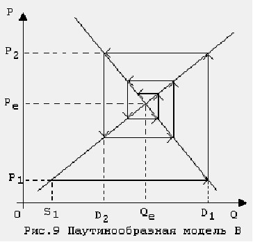
In the event of an imbalance between demand S1 and supply D1, the producer offers at the next time a product in the amount of S2 = D1, which he expects to sell at the price P2, determined from the condition S2 = S (P2), Then the process is repeated; graphically, it is convenient to present it in the form of a dynamic spiral depicted in Fig. 7.24.

Let’s consider the described iterative process in more detail. In the first step, at the price of P1, there is excess demand, as a result of which consumption is equal to supply. Since in this case the commodity is sold in the volume of S1, which is less than the equilibrium value of Qe, the commodity producer loses part of the profit, since the price, as it turned out, is underestimated, and less goods are offered than could be sold.

Lost profits force the commodity producer to increase the price of the goods and the volume of its supply. Assuming that demand will not change, he decides to increase output to the volume of D1. Supply at this volume is, as the producer hopes, optimal in the case when the price P2 satisfies the equation S(P2) = D1. This means that in the second step, the seller (aka the producer) sets prices using the supply curve.

Since the price of P2 corresponds to the demand for D2, then by virtue of D2<S2, the consumption in the second step is D2 (now part of the proposed product does not find a buyer due to the high price). As a result of this imbalance, the company again loses, not receiving a part of the profit.

To improve the situation on the market in this case, the firm must reduce supply and reduce the price. According to the assumptions used herein, supply should decrease to the demand level D2, and the price to the level P3, which is determined from the condition S(P3) = D2. Then the process is repeated.

Note that in model B, unlike model A, the dynamic spiral is “wound” already counterclockwise. Thus, the change in hypotheses about the behavior of the consumer and the commodity producer led to a change in the direction of movement in a spiral to the opposite. Therefore, in model B, with linear functions of supply and demand (5), price fluctuations fade and equilibrium is reached in the market at s>d.

If s<d, then in this case the price fluctuations increase, and at s = d, as in model A, prices fluctuate with a constant amplitude. As you can see, the change in the hypotheses of model A led not only to a change in the direction of the “winding” spiral, but also to a change in the condition of convergence of the iterative process to the opposite.

So, if the iterative process of price dynamics in one of the considered models converges, then in the other it diverges.

In conclusion, we consider the question of the correspondence of models A and B to the real process of consumption of goods. It is convenient to compare the main assumptions by summarizing them in Table 7.3.

Table 7.3.

As you can see, both of the considered models of the market of one product are vulnerable, since they are quite simple and do not take into account many factors contributing to the establishment of an equilibrium price.