The equilibrium ![]()
![]() price can be interpreted as a “fair” exchange price, which is established as a result of numerous paired transactions between sellers and buyers. This state of equilibrium is remarkable in that it is completely satisfied with demand, and there is no excessive production of goods, i.e. there is no overproduction of the product and irrational expenditure of production resources. Thus, from a production point of view, the equilibrium state corresponds to the greatest In this regard, the equilibrium state is acceptable and suitable for both groups of participants in the market exchange: producers and consumers; and therefore can act as the ultimate goal of the process of regulation by means of prices.
price can be interpreted as a “fair” exchange price, which is established as a result of numerous paired transactions between sellers and buyers. This state of equilibrium is remarkable in that it is completely satisfied with demand, and there is no excessive production of goods, i.e. there is no overproduction of the product and irrational expenditure of production resources. Thus, from a production point of view, the equilibrium state corresponds to the greatest In this regard, the equilibrium state is acceptable and suitable for both groups of participants in the market exchange: producers and consumers; and therefore can act as the ultimate goal of the process of regulation by means of prices.
As a rule, in a competitive economy without collusion (coalition), achieving equilibrium is a spontaneous process based on the fact that at any price exceeding the equilibrium price, the amount of goods that sellers (producers) seek to offer will exceed the amount for which buyers (consumers) intend to demand; there is downward pressure on the price, and the activities of some sellers who want to get rid of the goods will be directed against the existing (too high) price level. Similarly, it can be shown that a price below the equilibrium level is under upward pressure.
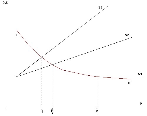
In the emergence and design of a stable demand for goods, depending on the price, i.e. the presence of the demand function D (p), which does not change in time, three main types of market equilibrium are distinguished, following A. Marshall:
1) instantaneous equilibrium is achieved in an environment where supply is fixed (![]()
![]() ), i.e. producers of goods are not ready to expand production or are not able to do so; equilibrium of this kind is usually achieved at a sufficiently high price
), i.e. producers of goods are not ready to expand production or are not able to do so; equilibrium of this kind is usually achieved at a sufficiently high price ![]() , which is the incentive for subsequent actions of producers;
, which is the incentive for subsequent actions of producers;
2) short-term equilibrium occurs when cash reserves (free production capacity) are put into operation and supply increases slightly, and ![]()
![]() the equilibrium price
the equilibrium price ![]() in this situation is lower
in this situation is lower ![]() , but also remains quite high;
, but also remains quite high;
3) a long-term normal equilibrium is established in a situation where almost all producers who are able to produce this product without a sharp restructuring of their economic activity take part in the business. The supply ![]()
![]() function is also an increasing and equilibrium price
function is also an increasing and equilibrium price ![]() corresponds to normal production costs (Figure 7.7).
corresponds to normal production costs (Figure 7.7).
The process of approaching the normal equilibrium in time can be represented using a sequence of small discrete steps, using ideas about the functions of supply and demand, which themselves can change during the market process due to changes in the conditions of production and consumption.
One of the main models of the process of achieving equilibrium uses its discrete representation using the so-called “trading” days with numbers. ![]()
![]()
Rice. 7.7. Prolonged normal equilibrium in the market
It is assumed that by the beginning of the trading day t the initial price of the goods ![]()
![]() is known, which completely determines the volume of supply
is known, which completely determines the volume of supply
![]()
![]() .
.
Further, it is considered that during the day the proposed goods are fully sold at a price ![]()
![]() that is determined from the condition of temporal equilibrium.
that is determined from the condition of temporal equilibrium.
![]()
![]()
and is the initial price for the next trading day (t+1), etc.
A geometric illustration of this process of approaching equilibrium (Fig. 7.8) resembles a spider web and therefore the model itself is often called a spider’s web. It can be shown that the convergence of the market process will be guaranteed if the following condition is met:
![]()
![]() .
.
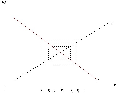
Rice. 7.8. Spider-like model
The latter means that it is sufficient for convergence that marginal supply does not exceed marginal demand, or, in other words, a positive reaction of the producer to a price increase would not be as significant as a negative reaction of the consumer, i.e. it is a process in an environment of relatively inactive producers. Note that if ![]()
![]() , then a situation of the so-called “pig cycle” arises, in which the equilibrium state is unattainable. If the slope of the demand line is steeper than the slope of the supply line, the spiral will unwind in reverse order. If the slopes of the supply and demand lines are the same, then the web will loop (Fig. 7.9)
, then a situation of the so-called “pig cycle” arises, in which the equilibrium state is unattainable. If the slope of the demand line is steeper than the slope of the supply line, the spiral will unwind in reverse order. If the slopes of the supply and demand lines are the same, then the web will loop (Fig. 7.9)
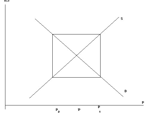
Rice. 7.9. Looped spider web model (equilibrium in the market is unattainable)
The second model of the process of achieving equilibrium, on the contrary, can be used to describe the situation of active producers who are ready to immediately respond to emerging demand. Such a process is set using the following system of relations: on trading day t, an offer ![]()
![]() is set and it determines the price
is set and it determines the price ![]() as a solution to the equation:
as a solution to the equation:
![]()
![]() .
.
This price characterizes the volume of demand
![]()
![]()
and the supply for the next trading day is directly guided by the demand of the previous day.
![]()
![]()
The described process can also be represented using a spider web model, and a sufficient convergence condition is:
![]()
![]()
which corresponds to a stronger reaction of producers compared to consumers. Let’s illustrate the discussed process of achieving equilibrium using the example that was presented earlier.
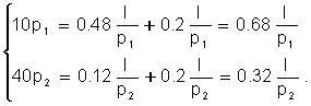
Let the function of the sentence be:
S(p) = 4p – 3,
and the demand function:

The main ratio is:
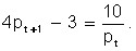
From here, the price on each subsequent market day is determined through the price on the previous day according to the formula:
Suppose that the initial price ![]()
![]() is , and summarize the results of the calculation in Table 7.1.
is , and summarize the results of the calculation in Table 7.1.
Table 7.1 Resource requirements by component
Convergence of price to equilibrium in time
p | D | S | E=D-S |
1,5 | 6,67 | 3 | 3,67 |
2,42 | 4,14 | 6,67 | -2,53 |
1,78 | 5,61 | 4,14 | 1,47 |
2,15 | 4,65 | 5,61 | -0,96 |
1,91 | 5,23 | 4,65 | 0,58 |
2,06 | 4,85 | 5,23 | -0,38 |
1,96 | 5,10 | 4,85 | 0,25 |
2,02 | 4,95 | 5,10 | -0,15 |
1,99 | 5,02 | 4,95 | 0,07 |
2,01 | 4,98 | 5,02 | -0,04 |
2,00 | 5 | 4,98 | 0,02 |
Thus, we see that after 11 “market” days, the price setting process converges to a state of equilibrium, and the equilibrium price ![]()
![]() value is already known to us. Note that the intermediate values of the price alternately become larger or less than the equilibrium value. This means that the process has an oscillatory character with a decreasing amplitude (Fig. 7.10).
value is already known to us. Note that the intermediate values of the price alternately become larger or less than the equilibrium value. This means that the process has an oscillatory character with a decreasing amplitude (Fig. 7.10).
Strictly monotonous is the process of achievement, known as “groping”, in which an important role is played by external (centralized) regulation. We will consider here one of the models of such a process, which bears the name of P. Samuelson. In this model, the price change is directly dependent on the amount of excess demand on trading day t:
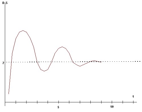
Rice. 7.10. The process of convergence of the price to the equilibrium
When (demand is greater than supply) the ![]()
![]() price rises, otherwise decreases. This process converges at any ratio between
price rises, otherwise decreases. This process converges at any ratio between ![]() . Its most common interpretation is that there is an arbitrator (auctioneer) in the market who evaluates the amount of residual demand and on the basis of this estimate declares the price (
. Its most common interpretation is that there is an arbitrator (auctioneer) in the market who evaluates the amount of residual demand and on the basis of this estimate declares the price (![]() ) for the next day, and all participants in the process strictly follow its instructions. Consumers form their demand in accordance with the demand function D (p), and manufacturers provide release according to the sentence function S(p). The value of a, which is called a tuning parameter, plays a big role in this scheme, because if its values are too small, the process converges very slowly, and if it is too large, it may not converge to equilibrium.
) for the next day, and all participants in the process strictly follow its instructions. Consumers form their demand in accordance with the demand function D (p), and manufacturers provide release according to the sentence function S(p). The value of a, which is called a tuning parameter, plays a big role in this scheme, because if its values are too small, the process converges very slowly, and if it is too large, it may not converge to equilibrium.
Let’s demonstrate the course of this process in the example above, and put the value of the parameter a = 0.1.
The main ratio is:
The results of calculations c ![]()
![]() are shown in Table 7.2.
are shown in Table 7.2.
Table 7.2 Resource requirements by component
“Groping” the equilibrium price according to the model of P. Samuelson
p | D | S | E=D-S |
1,5 | 6,67 | 3 | 3,67 |
1,87 | 5,35 | 4,48 | 0,87 |
1,96 | 5,11 | 4,83 | 0,28 |
1,99 | 5,03 | 4,96 | 0,07 |
2 | 5 | 5 | 0 |
To analyze the properties of such a controlled market process, a model in differential form can be used:
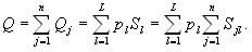
The equilibrium state in a complex market for many commodities can also be determined using supply and demand functions. Suppose that the market is an L of various products with numbers
l= 1, … , L. Denote through ![]()
![]() – the system of prices for goods;
– the system of prices for goods; ![]() – demand functions,
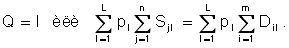
– demand functions, ![]() – supply functions. Then equilibrium in the narrow sense is the state in which the coincidence of supply and demand for all commodity items is realized:
– supply functions. Then equilibrium in the narrow sense is the state in which the coincidence of supply and demand for all commodity items is realized:
![]()
![]()
where ![]()
![]() is the system of equilibrium prices.
is the system of equilibrium prices.
Equilibrium in the broad sense should be considered any state for which:
![]()
![]()
The properties of the equilibrium state in the market of many goods are in many ways similar to the same state in the market of one commodity. However, in order to study it more thoroughly, it is useful to consider separately the markets for interchangeable and complementary goods.
In the case of the market for interchangeable goods, the demand functions satisfy the ratios:
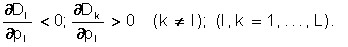
The last condition means that with an increase in the price of any product and the invariability of prices for other goods, the consumer sector will reduce its demand for it, but at the same time increase the demand for other, replacing it, goods.
The process of achieving equilibrium in this case can be represented by studying the sequence of “trading days”. At the same time, it is believed that by the beginning of the trading day (t + 1), the price ![]()
![]() system is known, which was formed earlier and served as a guide for manufacturers supplying goods to the market in quantities:
system is known, which was formed earlier and served as a guide for manufacturers supplying goods to the market in quantities:
![]()
![]()
During the trading day (t+1), there is a complete sale of goods and the new price ![]()
![]() system is determined according to the demand functions. In other words, the new price system is found as a solution to the system of equations:
system is determined according to the demand functions. In other words, the new price system is found as a solution to the system of equations:
![]()
![]()
It should be noted that the convergence of this process to the equilibrium position is ensured in the case when the condition is met:
![]()
![]() ,
,
where ![]()
![]() are the Jacobi matrices (composed of the first partial derivatives) for the supply and demand functions, respectively. In the course of successive exchanges, various methods of regulation can be used that make it possible to achieve equilibrium if convergence does not take place, or to accelerate the process of reaching equilibrium. In most cases, the cause of the irreducibility of the process is too high elasticity of supply at price, which causes violations of the above of sufficient condition. In order to reduce this elasticity, “underproduction incentives” are used, usually in the form of either direct compensation for low production or by sharply raising taxes for large volumes of production.
are the Jacobi matrices (composed of the first partial derivatives) for the supply and demand functions, respectively. In the course of successive exchanges, various methods of regulation can be used that make it possible to achieve equilibrium if convergence does not take place, or to accelerate the process of reaching equilibrium. In most cases, the cause of the irreducibility of the process is too high elasticity of supply at price, which causes violations of the above of sufficient condition. In order to reduce this elasticity, “underproduction incentives” are used, usually in the form of either direct compensation for low production or by sharply raising taxes for large volumes of production.
To describe the process of achieving equilibrium with centralized regulation (“groping”), the scheme mentioned above is used, which for the case of many goods has the form:
![]()
![]()
Here ![]()
![]() are the settings,
are the settings,
![]()
![]()
The use of the max sign avoids the appearance of negative price values.
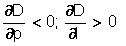
In the case of complementary (complementary) goods, their markets can be considered independently of each other. At the same time, the state of equilibrium on the demand side is largely determined by what share of its income the consumer sector allocates to the purchase of this product, and on the supply side it depends on the volume of resources that can be allocated to the production of this product.
Thus, we can assume that the demand function has the form:
D = D(p, I),
where p is the price of the goods;
I is the part of the consumer’s income allocated for its acquisition, and the ratios are fair
 . (*)
. (*)
The volume of demand is regulated by changing the specified share of consumer income.
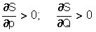
The sentence function is expressed as follows:
S = S(p, Q),
where Q is the amount of resources allocated to regulate the behavior of the producer.
At the same time, there are inequalities:
 . (**)
Based on the equilibrium condition:
![]()
![]()
and the ratios (*) and (**) obtain that the equilibrium ![]()
![]() price depends on the amount of resources (Q) and income (I) as follows:
price depends on the amount of resources (Q) and income (I) as follows:
 ,
,
 .
.
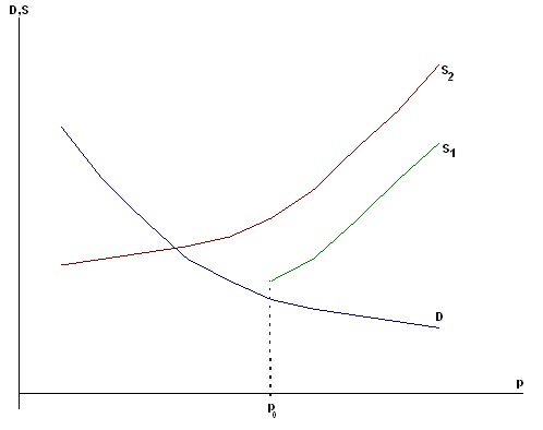
Thus, as the volume of resources increases on the production side (Q), the equilibrium price decreases with constant demand (see Figure 7.11), where the supply curve S1 corresponds to a fixed volume of the resource R, and the curve S2 corresponds to the increased volume (![]()
![]() ).
).
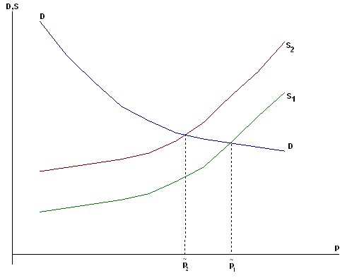
Rice. 7.11. As the volume of resources increases, the equilibrium price decreases
Similarly, with constant supply and an increase in consumer incomes, the demand curve D shifts to the right and the equilibrium price increases (Figure 7.12).
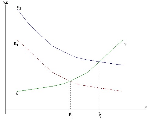
Rice. 7.12. The growth of consumer income shifts the demand curve upwards to the right
The results obtained can be used to develop methods of non-market regulation based on subsidies and subsidies. In some cases, the existence of equilibrium is not a matter of course, and its implementation requires additional efforts.
1) A situation in which the producer incurs high costs in the production process and therefore cannot start supplying products at a price below the margin of profitability (p0). However, this price is very high for consumers and demand at prices ![]()
![]() is less than the volume of production at which it is profitable (Figure 7.13).
is less than the volume of production at which it is profitable (Figure 7.13).
Rice. 7.13. Subsidizing the manufacturer allows to achieve equilibrium in the market
As can be seen, in this environment there is no equilibrium in the narrow sense, but there is an equilibrium in the broad sense of ![]()
![]() (supply more than demand). The position can be corrected by subsidizing the producer, after which the supply curve (S1) moves left to the position (S2) and the equilibrium point can be reached.
(supply more than demand). The position can be corrected by subsidizing the producer, after which the supply curve (S1) moves left to the position (S2) and the equilibrium point can be reached.
2) the case of shortage, when the production of goods is small and reacts weakly to an increase in price, i.e. almost or completely inelastic; and consumers are ready to purchase a large number of goods at almost any price (Fig. 7.14).
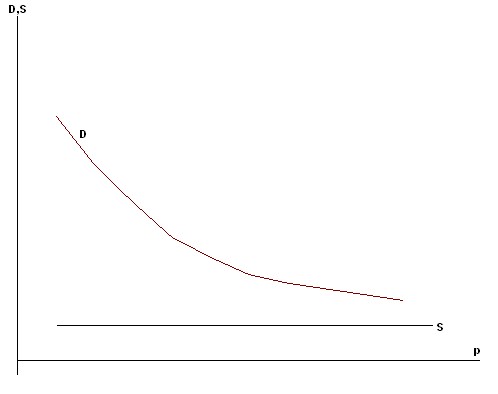
Rice. 7.14. With insufficient production of inelastic goods, there is no equilibrium in the market, there is a deficit
It is not difficult to see that in the field of reasonable prices there is no equilibrium either in a narrow or in a broad sense, on the contrary, there is a shortage of goods. Equilibrium can be achieved either by a sharp rise in production or by sharply limiting (restricting) consumer incomes, for example, monetary reform.
The properties of economic equilibrium in the markets of many goods can be studied using the following model of a closed economy.
Suppose there is an L of the product markets with the numbers l = 1, …, L ; m consumers (i = 1, …, m) and n producers (j = 1, …, n). The vector ![]()
![]() represents a system of prices for goods; through
represents a system of prices for goods; through ![]() the demand of the i-th consumer for the l-th product is indicated, through
the demand of the i-th consumer for the l-th product is indicated, through ![]() the supply of the l-th product by the manufacturer with the number j. The group of equilibrium conditions for each product has the form:
the supply of the l-th product by the manufacturer with the number j. The group of equilibrium conditions for each product has the form:
 . (***)
We also propose, as before, that the demand functions depend on the price system and on the income of the consumer (Ii):
![]()
![]()
Supply functions are expressed through the price system and the financial resource of the producer (Qj):
![]()
![]()
For given incomes (Ii) and resources (Qj), the L system of equations (***) is used to find the equilibrium price system:
![]()
![]()
It can be shown that the existence of an economically meaningful (non-negative) equilibrium system of prices is associated with the fulfillment of an additional condition on the ratios of incomes of consumers (Ii) and resources of producers (Qj).
In the future, we will proceed from the fact that the total income of (i) consumers is fully spent on the purchase of goods.
and the total resource (Q) of producers is obtained as a result of the sale of goods
The following two cases are possible:
(a) The aggregate values indicated shall be equal to each other:
 (****)
This situation is obtained as a result of the normal operation of a self-sustaining system of markets, in which the monetary demand (Q) from producers is fully satisfied at the expense of consumer spending (I). Under natural assumptions about the functions of supply and demand (see above), the system of equations (***) taking into account (****) makes it possible to find an equilibrium price system with an accuracy of a constant multiplier, i.e. a system of relative prices. For convenience, one of the goods is usually taken as a basic (for example, money) or simply called a unit of account (its price is 1).
b) the total income of consumers and the income of producers are not equal to each other:
![]()
![]()
In this case, the system of equations (***), generally speaking, has no non-negative solution, i.e. there is no economically meaningful system of equilibrium prices.
Consider the following example of a two-product market in which there are two producers (each supplying only one product) and two consumers (each using both).
Let be ![]()
![]() the prices of goods:
the prices of goods:
1) the functions of the offer have the form:
![]()
![]()
Thus, the total income of producers
![]()
![]()
(2) Demand functions are expressed as follows:
total income of consumers:
![]()
![]()
Income of the first consumer:
![]()
![]()
Income of the second:
![]()
![]()
Functions of the demand of the first consumer for goods, respectively:
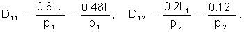
Functions of demand of the second consumer:
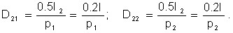
Equilibrium condition:
Hence we have the ratio of equilibrium prices:
![]()
![]()
If we take the second product as the base (the unit of account is the ruble), and express the physical volumes of goods in tons, then the equilibrium state in the markets is as follows:
prices ![]()
![]() = 2.915 rubles / ton;
= 2.915 rubles / ton;
![]()
![]() = 1 rub./ton;
= 1 rub./ton;
production of the first product
S1 = 29.15 tonnes;
second product
S2 = 40 tons;
consumer purchases:
D11 = 20.62 t ; D12 = 15 t;
D21 = 8.59 t ; D22 = 25 tons;
total income of producers:
R = 125 thousand rubles;
Consumer spending:
I1 = 75 thousand rubles; I2 = 50 thousand rubles.
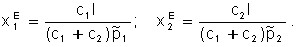
In conclusion, consider the equilibrium model, in which the set of production capabilities of the enterprise (Fig. 7.15) is set using the ratio:
At the same time, the company seeks to maximize gross income:
![]()
![]() .
.
The solution to this problem is:
These expressions give us the dependence of supply on prices (supply ![]()
![]() functions).
functions).
![]()
![]()
subject to budget constraints:
![]()
![]()
The solution to this problem is as follows:
It represents the demand ![]()
![]() functions of .
functions of .
Equilibrium conditions are presented in the following form:
![]()
![]()
Solving the resulting system of equations with respect ![]()
![]() to , we obtain the value of equilibrium prices:
to , we obtain the value of equilibrium prices:
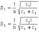 ,
,
and the coordinates of the equilibrium point E:
Point E touching the boundary of the set of production possibilities and the highest achievable indifference curve is the Pareto optimum. The line PQ separating these sets is called the price line.
The process of achieving equilibrium is carried out here by the simultaneous movement of the consumer and the producer.
The consumer reaches the highest level of utility at point E by moving along the price line, i.e. being within the budget constraint (Figure 7.15).
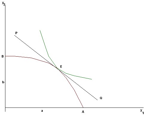
Rice. 7.15. Optimum according to Pareto
The producer reaches the highest level of profit at point E, moving along the boundary of the many production capabilities of AB.