The study of modern production shows that each phenomenon is in close interrelation and interaction.
When studying specific dependencies, some signs act as factors that cause a change in other signs. The signs of this group are called signs-factors (factor signs), and the signs that are the result of the influence of these factors are called effective (as the volume of output is affected by the technical equipment of production, then the volume of production is effective, and the technical equipment is a factor feature). There are two types of dependencies between economic phenomena – functional and stochastic. With the functional connection of each specific system of values of factor features, one or more strictly defined values of the effective feature correspond. Examples of functional dependence can be given from the field of physical phenomena (S = v· t).
Stochastic (probabilistic) connection is manifested only in mass phenomena. In this relationship, each particular system of values of factor features corresponds to some set of values of the effective feature. A change in factor features does not lead to a strictly defined change in the effective feature, but to a change only in the distribution of its values. This is due to the fact that the dependent variable, in addition to the selected variable, is subject to a number of uncontrolled or unaccounted factors, and also because the measurement of variables is inevitably accompanied by some random errors. Since the values of the dependent variable are subject to random variation, they cannot be predicted with sufficient accuracy, but only indicated with a certain probability (number of defective parts per shift, number of downtime per shift, etc.).
Stochastic connection is called correlational. Correlation in the broad sense of the word means a connection, a relationship between objectively existing phenomena and processes. Regression is a special case of correlation. While correlation analysis estimates the strength of the stochastic connection, regression analysis examines its shape, i.e. there is a correlation equation (regression equation).
Consider the different types of correlation and regression.
According to the number of variables, regression is distinguished:
1) pair – regression between two variables (profit ![]()
![]() productivity);
productivity);
2) multiple – regression between the dependent variable y and several variables ![]()
![]() (labor
(labor ![]() productivity, the level of mechanization of production, the qualifications of workers).
productivity, the level of mechanization of production, the qualifications of workers).
Regarding the form of dependence, the following are distinguished:
linear regression; nonlinear regression.
Depending on the nature of the regression, the following are distinguished:
1) direct regression. It occurs if, with an increase or decrease in the values of factor variables, the values of the effective variable also increase or decrease;
2) reverse regression. In this case, with an increase or decrease in the values of the factor trait, the effective trait decreases or increases.
Regarding the type of compounds of phenomena are distinguished:
1) direct regression. In this case, the phenomena are connected directly to each other (profit ![]()
![]() costs);
costs);
2) indirect regression. It occurs if the factor and resulting variables are not directly causal and the factor variable acts on the effective variable (number of fires and grain yield (meteorological conditions)) through some other variable;
3) false or absurd regression. It arises with a formal approach to the phenomena under study. As a result, it is possible to come to false and even meaningless dependencies (the number of imported fruits and the increase in road accidents with a fatal outcome).
The classification and correlations are similar.
The study of interdependencies in economics is of great importance. Statistics not only answers the question of the real existence of a connection between phenomena, but also gives a quantitative description of this dependence. Knowing the nature of the dependence of one phenomenon on another, it is possible to explain the causes and size of changes in the phenomenon, as well as to plan the necessary measures for its further change. In order for the results of correlation analysis to find practical application and give the desired result, certain requirements must be met:
1) homogeneity of units subject to correlation analysis (enterprises produce the same type of products, the same nature of the technological process and the type of equipment);
2) a sufficient number of observations;
3) the factors included in the study should be independent of each other.
Balance and index methods are used to study functional relationships. To study stochastic relationships, the parallel series method, the method of analytical groupings, variance analysis and analysis of regressions and correlations are used.
The simplest method of detecting connections is to compare two parallel series. The essence of the method is that first the indicators characterizing the factor feature are ranked, and then the corresponding indicators of the effective feature are located parallel to them. Comparison of rows constructed in this way makes it possible not only to confirm the very presence of a connection, but also to identify its direction.
In the case where the series being compared consists of a large number of units, the communication directions for different units may be different. In this case, it is more expedient to use correlation tables. In the correlation table, the factor feature (x) is placed in rows, and the effective (y) is placed in columns. The numbers located at the intersection of the rows and columns of the table show the frequency of repetition of this combination of x and y. The construction of the correlation table begins with the grouping of observation units by the values of factor and effective features. If the frequencies in the correlation table are arranged diagonally from the upper left coal to the lower right corner, then we can assume the presence of a direct correlation relationship. If the frequencies are located diagonally from right to left, then they assume the presence of a feedback relationship between the signs.
Another method of detecting a relationship is to build a group table (the method of analytical groupings). The totality of the values of factor x is divided into groups and for each group the average value of the effective feature is calculated. It is assumed that with a sufficiently large number of observations in each group, the influence of other random factors in calculating the group average will be mutually canceled and the dependence of the effective feature on the factor feature will be more clearly revealed and, consequently, the differences in the value of the averages will be associated only with differences in the value of this factor feature. If there were no relationship between the factor and the scoring trait, then all group averages would be approximately the same in magnitude.
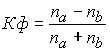
The simplest indicator of the closeness of the connection is the coefficient of correlation of signs (G. Fechner coefficient):
 ,
,
where ![]()
![]() is the number of coincidences of the signs of deviations of the individual value from the average;
is the number of coincidences of the signs of deviations of the individual value from the average;
![]()
![]() is the number of mismatches of the deviation signs of the individual value from the average.
is the number of mismatches of the deviation signs of the individual value from the average.
This coefficient allows you to get an idea of the direction of communication and an approximate characteristic of its closeness. To calculate it, the average values of the effective and factor features are calculated, and then deviation signs are put for all values of the interrelated features Kf = [-1; +1]. If the signs of all deviations coincide, then ![]()
![]() Kf = 1 is a direct relationship, if the signs of all deviations are different, then Qf = – 1, which indicates the presence of feedback.
Kf = 1 is a direct relationship, if the signs of all deviations are different, then Qf = – 1, which indicates the presence of feedback.
Table 28 Resource requirements
Number of employees and balance sheet profit
Number of workers, people.
| Balance sheet profit, thousand rubles
| Sign of deviations of the individual value of the feature from the average | Match (a), mismatch (b) | |
|
| |||
304 | -258 | + | – | b |
269 | 459 | + | + | a |
212 | 261 | – | – | a |
165 | 604 | – | + | b |
141 | 356 | – | + | b |
![]()
![]() People
People
![]()
![]() thousand rubles.
thousand rubles.
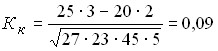
![]()
![]() , thus, there is little feedback between the signs.
, thus, there is little feedback between the signs.
To approximate the direction and closeness of the relationship between the features represented by the two series, you can also use the rank correlation coefficient. When determining the coefficient of correlation of ranks, the values x are ranked, and then the corresponding values of y are ranked. As a result, we get ranks, i.e. places, numbers of units of the population in an ordered series. At the same time, if there are identical variants, each of them is assigned an arithmetic mean of their ranks.
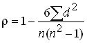
Spearman’s rank correlation coefficient:
 ,
,
where d is the difference between the ranks of the corresponding values of the two features;
n is the number of units in the row.
The rank correlation coefficient takes values [-1; 1]. If ![]()
![]() there is a close direct relationship,
there is a close direct relationship, ![]() a close feedback,
a close feedback, ![]() there is no connection. The rank correlation coefficient has certain advantages over other characteristics of the direction and closeness of the connection: it can be determined by examining data that are not amenable to numbering, but are ranked (shades, quality).
there is no connection. The rank correlation coefficient has certain advantages over other characteristics of the direction and closeness of the connection: it can be determined by examining data that are not amenable to numbering, but are ranked (shades, quality).
For the numerical characterization of the closeness of the bond, indicators of variation of the resulting feature can be used: its total variance ![]()
![]() and intergroup variance (
and intergroup variance (![]() ).
).
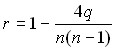
Kendel’s rank correlation coefficient:
 ,
,
where q is the number of ranks arranged in reverse order.
In the practice of statistical research, it is often necessary to analyze alternative distributions, when the population is distributed for each feature into two groups with opposite characteristics. The closeness of the connection in this case can be estimated using the coefficient of contingence:
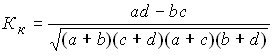 .
.
Table 29 Resource requirements
The dependence of student performance on gender
Contingent of students | Altogether | ||
who passed the exams | who have not passed the exams | ||
women | a = 25 | b = 2 | a + b = 27 |
men | c = 20 | d = 3 | c + d = 23 |
Total | a + c = 45 | b + d = 5 | 50 |
 .
.
Consequently, there is practically no connection between the gender of the student and his academic performance.
The association coefficient is calculated as follows:
![]()
![]() .
.
The previously considered statistical methods for studying relationships are often insufficient, because they do not allow to express the existing connection in the form of a certain mathematical equation. Methods of parallel series and analytical groupings are effective only with a small number of factor features, while socio-economic phenomena usually develop under the influence of many reasons. These limitations are eliminated by the method of correlation and regression analysis.
The method of analyzing correlations and regressions is to build and analyze an economic-mathematical model in the form of a regression equation, expressing the dependence of the phenomenon on the factors determining it. For example, the dependence of the volume of production (y) (million rubles) on its technical equipment (x) (%) is expressed by the following dependence:
![]()
![]() .
.
It can be assumed that with an increase in technical equipment by 1%, the volume of production will increase by an average of 21.4 million rubles.
The method of correlation and regression analysis consists of the following steps:
preliminary analysis; collection of information and its primary processing; building a model (regression equations); Evaluation and analysis of the model.
At the first stage, it is necessary to formulate the task of the study in a general form (studying the influence of various factors on the level of labor productivity). Next, it is necessary to determine the methodology for measuring the effective indicator (labor productivity can be determined by natural, labor or cost methods). It is also necessary to determine the number of factors that have the most significant impact on the formation of an effective feature.
At the stage of collecting and processing information, the researcher needs to remember that the studied population should be large enough in volume. The initial data should be qualitatively and quantitatively homogeneous.
When building a correlation model (regression equation), the question arises about the type of analytical function that characterizes the mechanism of the relationship between the features. This relationship can be expressed by:
a straight line ![]()
![]() ; a second-order
; a second-order ![]() parabola; a hyperbola; an
parabola; a hyperbola; an ![]() exponential function
exponential function ![]() , etc.
, etc.
That is, the question arises about the choice of the form of communication. The type of empirical regression suggests what type of curve can be described. Next, the regression equation is solved. Then, with the help of special criteria, their adequacy is assessed and the form of communication that provides the best approximation and sufficient statistical reliability is selected. Having chosen the form of the connection and having built the regression equation in a general form, it is necessary to find the numerical value of its parameters. To find the parameters, use the method of least squares. Its essence is as follows:
![]()
![]() ,
, ![]()
![]()
![]() .
.
There are partial derivatives of this expression by ![]()
![]() and
and ![]() are equated to zero. After the transformations, we get a system of normal equations:
are equated to zero. After the transformations, we get a system of normal equations:
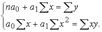
The solution of this system in general form gives the following parameter values:
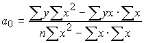
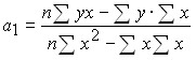 .
.
After finding the parameters, we obtain the regression equation, by which we find the theoretical frequencies ![]()
![]() for each value
for each value ![]() of .
of .
You can get ![]()
![]()
![]() it in another way. Let’s divide the normal equation
it in another way. Let’s divide the normal equation ![]() by
by ![]() and we get:
and we get:
![]()
![]()
![]()
![]()
![]()
![]() .
.
The regression coefficient can be represented as follows:
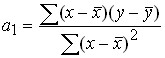 .
.
The regression ![]()
![]() coefficient shows the measure of the effect of the change in the explanatory variable x on the dependent variable y. The regression
coefficient shows the measure of the effect of the change in the explanatory variable x on the dependent variable y. The regression ![]() constant determines the intersection point of the line regression with the ordinate axis. After determining the estimates
constant determines the intersection point of the line regression with the ordinate axis. After determining the estimates ![]() of the regression
of the regression ![]() parameters and
parameters and ![]() , as well as the values,
, as well as the values, ![]() we define a random variable
we define a random variable![]() . It characterizes the deviation of the
. It characterizes the deviation of the ![]() variable from the value of .
variable from the value of .
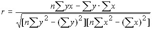
In the linear form of communication, the indicator of its closeness is the linear correlation coefficient:
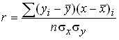 ,
,
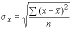 ;
; 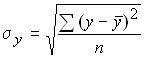 ;
;
 .
.
The correlation coefficient takes values [-1; +1]: r = –1 – inverse relationship; r = +1 is a straight line.
Knowing the linear correlation coefficient, it is possible to determine the regression coefficient (![]()
![]() ) in the regression equation
) in the regression equation
![]()
![]() , then .
, then . 
Security questions
The essence of the stochastic relationship between phenomena. What is correlation? Provide a classification of the regression. The main methods of detecting the relationships between phenomena. How to build a correlation table? When is the association coefficient calculated? The main stages of correlation-regression analysis. How to determine the linear correlation coefficient?