As a result of statistical observation, “raw” material, records of individual units of observation are obtained. This material is not suitable for direct use for either practical purposes or scientific analysis. There is a need for special processing of statistical data, i.e. in the summary of observation materials.
The summary is a set of sequential actions to summarize specific single data that form a set in order to identify typical features and patterns inherent in the phenomenon under study as a whole.
The task of the summary is to characterize the subject under study with the help of systems of statistical indicators , to identify and measure its essential features and features.
A statistical summary is carried out according to a specific program. To develop a summary program means to determine which groups and subgroups will be allocated in the studied population, which indicators in the form of totals, averages or relative values should be calculated for the selected groups and in general for the population, in which tables the result of the summary will be formatted.
When developing a program, a statistical subject and a statistical predicate are determined. The subject is the object of study, divided into groups and subgroups. Predicates are statistical indicators that characterize the subject of the summary.
In terms of the depth of material processing, the summary is simple and complex. A simple summary is an operation to calculate the total totals for the aggregate. A complex summary is a set of operations that include grouping observation units, counting the totals for each group and for the entire object, and presenting the results of the grouping and summary in the form of statistical tables.
According to the form of material processing, the summary can be centralized and decentralized. With a centralized summary, all observation material is concentrated in one central organ and processed there. With a decentralized summary, the observation material is processed at several stages (the report of the production association of the district ![]()
![]() of the region
of the region ![]() results for the region
results for the region ![]() of the republic).
of the republic).
According to the technique of execution, the summary can be manual and mechanized (currently – dominant).
Groupings are the most important statistical method of summarizing data, the basis for the correct calculation of statistical indicators.
The division of a population into groups that are homogeneous in any way is called a grouping. Grouping is the centerpiece of any summary. It is thanks to groupings that the observation material takes on a systematized form.
For the first time in statistics, D.P. Zhuravsky paid due attention to the method of groupings. He considered the main method of analysis to be the selection and study of “monokind parts”, categories and groups.
The signs underlying the grouping are called grouping.
The whole set of signs can be divided into two groups: factor and effective. The relationship between them is manifested in the fact that with an increase in the value of a factor trait, the average value of the effective one systematically increases or decreases.
Grouping features can be of a different nature:
1) they can have a quantitative expression (age, wages, volume of output). These features are called quantitative, and groupings built on these features are called variation series;
2) qualitative signs (social status, profession, gender, nationality). Groupings built on these features are called attributive distribution series;
3) territorial characteristics (grouping of the population by regions, grouping of enterprises by districts). Groupings built on such grounds are called geographical or territorial series;
4) a sign of time (grouping of data about the object for a number of years). Groups built on such grounds are called rows of dynamics.
By dividing the population into parts and determining the number by groups, the following tasks can be solved with the help of groupings:
show the structure of the population; identify the main types and forms of the phenomenon; to identify the relationship between the phenomena.
Groupings in which the first task is solved are called structural (Table 2). Structural grouping is a grouping in which the population is divided into groups that characterize its structure according to some varying feature. With the help of such groupings, the composition of the population by sex, age, place of residence, the composition of enterprises by the number of employees, by the cost of fixed production assets, etc. can be studied.
Table 2 Resource requirements by component
Distribution of the employed population by sectors of the economy (as a percentage of the total)
Industries | Number of employed population, as a percentage of the total |
Total employed in the economy | 100 |
including: | |
industry | 28 |
agriculture | 15 |
construction | 8 |
transport and communications | 7 |
trade and catering | 11 |
health, physical education and social security | 7 |
education | 10 |
Other | 14 |
The groupings by which the second task is solved – the allocation of the main types and forms of the phenomenon, are called typological (Table 3). Typological grouping is the division of the studied population into qualitatively homogeneous groups.
Table 3 Resource requirements by component
Housing stock
(at the end of the year, millions of square meters of total area)
1990 | 1999 | |
Entire housing stock | 182,4 | 208,2 |
on average per inhabitant, m2 | 17,9 | 20,8 |
Urban housing stock | 106,4 | 131,5 |
on average per inhabitant, m2 | 15,5 | 18,8 |
Rural housing stock | 76,0 | 76,7 |
on average per inhabitant, m2 | 22,6 | 25,3 |
Groupings by which the relationship between phenomena is revealed are called analytical.
Features of analytical groupings are as follows:
the grouping is based on a factor feature; each selected group is characterized by the average values of the effective feature.
Analytical groupings make it possible to study the diversity of relationships and relationships between variable features. The advantage of the method of analytical groupings over other methods of communication analysis is that it does not require compliance with any conditions for its application, except for one – the qualitative homogeneity of the studied population.
In the construction of such groupings, of two or more interrelated indicators, one is considered as a factor (i.e., affecting the other), and the second as a result of the influence of the first. To identify the relationship between the indicators, it is necessary to ungroup the units of the population by factor feature and for each selected group to calculate the average value of the effective indicator and follow its changes (Table 4).
Table 4 Resource requirements by component
Grouping of enterprises by level of labor productivity and cost of production
Groups of enterprises by the level of labor productivity of one employee (thousand rubles) | Quantity Enterprises | Unit cost of production (thousand rubles) |
1000-1200 | 4 | 920 |
1200-1500 | 5 | 890 |
1500-1900 | 3 | 840 |
1900-2400 | 2 | 780 |
Statistical grouping can be made by one or more characteristics. Grouping by one feature is called simple, grouping by several signs is called combination (complex).
Complex grouping is called a grouping in which the division of the population into groups is made according to two or more features taken in combination.
Combination groupings allow a deeper analysis of the development of phenomena, interrelations and dependencies between them. Combination is the grouping of the population by sex and age, the grouping of fixed assets by industry with the division of each group by natural-material composition (buildings, structures, etc.). However, it should be remembered that excessive fragmentation of groups can only complicate the analysis of the material. With the correct, scientific application of combination groupings, they are a very important and effective means of summarizing and analyzing statistical data.
A special type of groupings are groupings-classifications. Examples of classifications can serve as groupings of enterprises by industry, fixed assets – by type, production costs – by items, etc. It is characteristic of the classification that they are produced according to the most essential features that determine other signs and features of the phenomenon under study. Classifications are of great importance in statistics. When developing a classification, not only the characteristics and intervals of classification are determined, but it is also clearly established which units should be assigned to each group. The stability of the features and intervals by which the classification is carried out makes it possible to compare data for a number of years not only for the population as a whole, but also for its individual groups.
The most important classification groupings in domestic statistics are:
grouping of enterprises by forms of ownership; grouping (classification) of branches of the national economy; classification of industries; classification of fixed assets; classification of employees by categories of personnel (professions); cost classification; grouping of enterprises according to the degree of implementation of the plan; grouping of enterprises by size, etc.
Classifications are historical in nature: over time, new classifications appear or changes are made to previously existing classifications.
Secondary grouping is the regrouping of previously grouped data. The need for secondary grouping arises in two cases:
1) when the previously produced grouping does not satisfy the objectives of the study in relation to the number of groups;
2) to compare data relating to different territories and time periods, if the primary grouping was carried out according to different grouping features or at different intervals.
Two methods of secondary grouping are used:
combining the initial intervals; allocation of a certain proportion of units of the population (fractional rearrangement).
The following data are available on the grouping of enterprises by the cost of fixed production assets (OPF) (Table 5).
Table 5 Resource requirements by component
Grouping of enterprises by the cost of fixed production assets
Groups of enterprises at the cost of OPF, mln. rub. | Number of enterprises, as a percentage of the total | Volume of production, mln. rub. |
up to 5 | 5,0 | 150,2 |
5-10 | 6,2 | 240,0 |
10-20 | 13,6 | 450,2 |
20-40 | 14,2 | 486,2 |
40-60 | 18,0 | 524,0 |
60-100 | 25,4 | 650,2 |
100-150 | 10,2 | 880,4 |
150-250 | 4,4 | 990,0 |
250 and up | 3,0 | 895,0 |
Total | 100 | 5266,2 |
For the purposes of analysis, the following groups of enterprises should be distinguished by the cost of fixed production assets (million rubles): up to 20; 20-50; 50-100; 100-200; 200 and above. The result of the secondary grouping is given in Table 6.
Table 6 Resource requirements by component
Grouping of enterprises by the cost of fixed production assets
Groups of enterprises at the cost of OPF, mln. r. | Number of enterprises, as a percentage of the total | Volume of production, mln. rub. |
up to 20 | 5 + 6,2 + 13,6 = 24,8 | 150,2 + 240,0 + 450,2 = 840,4 |
20-50 | 14,2 + | 486,2 + |
50-100 |
|
|
100-200 | 10,2 + | 880,4 + |
200 and up |
|
|
Total: | 100 | 5266,2 |
After determining the grouping feature, the question of the number of groups into which the studied population should be divided should be solved. The number of groups depends on the tasks of the study and the type of feature underlying the grouping, the size of the population, the degree of variation of the trait.
Quantitative values of the feature, on the basis of which the studied phenomena that lie within certain boundaries are divided into groups and are called intervals in statistics. The meaning and significance of the intervals in the grouping depend on its ultimate goal, on the functions of the grouping feature and its relationship with other features, on the tasks of the study, on the features of the aggregate.
Each interval has its own size, upper and lower boundaries, or at least one of them.
The lower boundary of the interval is the smallest value of the feature in the interval; top – the largest value of the feature in it.
The size of the interval is the difference between the upper and lower boundary of the interval.
Grouping intervals can be equal and unequal. Equal intervals are used where it is necessary to show what quantitative differences exist within groups of the same quality, when the trait changes more or less evenly within limited limits. Equal intervals are established mechanically, by calculation according to the following formula:
![]()
![]()
![]() , or (1)
, or (1)
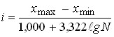 (Sturgess’ formula) (2)
where: ![]()
![]() ,
, ![]() is the maximum and minimum value of the feature in the aggregate;
is the maximum and minimum value of the feature in the aggregate;
n is the number of groups;
N is the size of the population.
Sturgess’s formula has a drawback. It gives good results with a large volume of the population and if the distribution of units by grouping feature is close to normal.
Equal intervals are used in cases where the ratio of the maximum and minimum values of the grouping feature does not exceed ten times the value.
In the case of a significant variation in the grouping feature, it is advisable to use multiple intervals (doubled intervals).
The value obtained by the formula is rounded. It is an interval step. There are the following rules for determining the interval step:
if the value of the interval is a value having one decimal place (for example, 7.35), then it is advisable to round the resulting values to tenths and use them as an interval step (7.4); If the interval value has two significant digits before the comma and slightly after the decimal point (15.671), then this value should be rounded to an integer (16); if the value of the interval is a three-, four-, and so on number, then this value must be rounded to the nearest number, a multiple of 100 or 50 (389 ≈ 400).
Example.
There are data on 10 enterprises for the production of products (million rubles): 16.2; 17,9; 15,4; 21,5; 18,1; 12,0; 14,9 13,8; 24,0 19,2. Make a grouping of enterprises by output, highlighting 6 groups with equal intervals.
Let’s determine the size of the interval:
i = ![]()
![]() = 2 million rubles.
= 2 million rubles.
To determine the upper limit of the first interval, add the amount of the interval to ![]()
![]() it (Table 7).
it (Table 7).
When grouped on a quantitative basis, the boundaries of the intervals can be marked in different ways. If the basis of the grouping is a continuous feature, then the same value of the feature acts as both the upper and lower boundaries at two symmetrical intervals. If the grouping is based on a discrete feature, then the lower boundary of the i-th interval is equal to the upper boundary of the i-1 interval increased by one.
Table 7 Resource requirements by component
Grouping of enterprises by production
Groups of enterprises for the production of products, million rubles. | Number of companies |
12,0 – 13,9 | 2 |
14,0 – 15,9 | 2 |
16,0 – 17,9 | 2 |
18,0 – 19,9 | 2 |
20,0 – 21,9 | 1 |
22,0 – 24,0 | 1 |
Altogether | 10 |
In economics, it is more common to use unequal, progressively increasing intervals. The use of unequal intervals is due to the fact that with their help the boundaries of qualitative transitions are taken into account, i.e. groups that are qualitatively distinguished from each other are distinguished.
The magnitude of the intervals varying in the arithmetic progression is determined ![]()
![]() by .
by .
Exponentially – ![]()
![]() ,
,
where ![]()
![]() =const is the number that will be positive at progressively increasing intervals and negative at progressively decreasing intervals;
=const is the number that will be positive at progressively increasing intervals and negative at progressively decreasing intervals;
![]()
![]() =const is a positive number that will be greater than 1 at progressively increasing intervals, and less than 1 at progressively decreasing intervals.
=const is a positive number that will be greater than 1 at progressively increasing intervals, and less than 1 at progressively decreasing intervals.
In groupings that are intended to display the qualitative originality of groups, specialized intervals are used. In this case, each group has its own special content, and the boundary of the interval is established where the transition from one quality to another occurs (Table 8).
Table 8 Resource requirements by component
Characteristics of the attitude of the male population of the CIS
to work
0 – 15 years | – disabled |
16 – 18 | – Persons of semi-working age |
19 – 59 | – Persons of working age |
60 – 69 | – Persons of semi-working age |
70 and older | – disabled |
Group intervals can be closed when the lower and upper boundaries are specified (Table 9).
Table 9 Resource requirements by component
Daily mileage of motor vehicles
Enterprise
Daily mileage (km) | Number of cars |
130 – 158 | 3 |
159 – 186 | 4 |
186 – 214 | 6 |
214 – 242 | 2 |
Total: | 15 |
Group intervals can be open when only one of the group boundaries is specified (see Table 8 – 70 years and older). Open intervals apply only to extreme groups. When grouping with unequal intervals, it is desirable to form groups with closed intervals, because this contributes to the accuracy of statistical calculations. The width of the open interval is taken to be equal to the width of the adjacent interval.
The variation of a feature in a row can be discrete (discontinuous) and continuous. With discrete variation, the values of the variants differ from each other by a well-defined amount and are usually expressed in integers. With a continuous variation of a feature, its value can take any value in a certain interval (see Table 9).