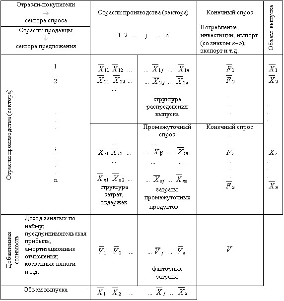
Cross-sectoral analysis is based on the use of statistical tables called “cross-sectoral”. The table of intersectoral balance describes the flows of goods and services between all sectors of the national economy during a fixed period of time (usually 1 year). The cross-sectoral balance sheet, expressed in terms of values, can be interpreted as a system of national accounts. You can easily imagine the structure of this kind of tables by looking at an example.
In the cross-sectoral balance for a country or region that trades with foreign countries, exports can be represented by positive, and imports negative – components of final demand.
The rows in the table show the output distribution of each product. Each line is characterized by the following balance:
Output of this type of product = Intermediate demand + Final demand
which can be mathematically written as:
| (9-1) |
Intermediate demand is a part of the total demand, which is the purchase of this type of product by industries 1, 2, 3, and so on as starting materials, i.e. as intermediate products. On the contrary, final demand is a product directed to the field of final use, i.e. it is distributed to non-industrial sectors of the economy. This includes the personal consumption of the population, the cost of maintaining the state apparatus, education, health care and so on.
The columns of the table show the input structure or the structure of the resources used that are required for each industry. The columns are set to the following balance:
Industry Costs = Intermediate Costs + Value Added,
which in a mathematical notation looks like this:
| (9-2) |
Intermediate costs are raw materials purchased by the industry from sectors 1, 2, 3, and so on. Value added is the factor costs of an industry, that is, newly created value that breaks down into the income of employees (wages) and entrepreneurial income (profit).
The rows and columns in the interdisciplinary balance sheet have the following identities:
Industry Output = Industry Expenses
Total amount of final demand = Total amount of value added,
which are mathematically written as follows:
| (9-3) | |
| (9-4) |
Now let’s look at the balance scheme in terms of its large components. There are several blocks with different economic content – quadrants of the balance.
In the first quadrant:
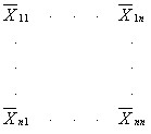
contains intersectoral flows of means of production (intermediate costs, production sector). In shape, it is a square matrix. The data of this quadrant play a decisive role in the analysis of the structure of material costs of industries, the proportions and production links between industries, flows in the material supply system.
In the second quadrant:
![]()
![]()
the final products of all branches of material production are presented. In the detailed balance sheet scheme, the final output of each industry is shown differentiated by areas of use: for personal consumption of the population, public consumption (governing bodies, education, sciences, and so on), for accumulation, and more. The second quadrant characterizes the sectoral material structure of national income, its distribution to the accumulation fund and the consumption fund.
Third Quadrant:
![]()
![]()
also characterizes national income, but on the part of its value composition. The elements of the third quadrant are the value equivalent of the final product, in foreign literature these elements are called primary costs. In the detailed balance sheet scheme, this quadrant contains various types of income of workers in material production. The data of the third quadrant are necessary for the analysis of the relationship between the newly created and transferred value, between the value of the necessary and surplus product in general for material production and in the sectoral context.
Note that the overall results of the second and third quadrants are:
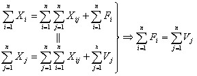
Thus, in the intersectoral balance, the most important principle of the unity of the material and value composition of national income is observed.
Fourth Quadrant:
![]()
![]()
reflects the final distribution and use of national income. As a result of the redistribution of the primary created national income, the final incomes of the population, enterprises, and the state are formed. Their value determines the share of participation of the population, state and other enterprises and institutions in the consumption and accumulation of the entire mass of final products. The data of this quadrant are important for reflecting in the cross-sectoral model the balance of incomes and expenditures of the population, sources of financing capital investments, for analyzing the general structure of final incomes by consumer groups.
In general, the intersectoral balance within the framework of a single economic and mathematical model combines the balances of the branches of material production, the balance of the entire social product, the balances of national income, the financing of incomes and expenditures of the population.
Along with the intersectoral balance in value terms, as already noted, inter-product balances in physical terms are being developed. The natural balance contains a list not of industries, but of the products of material production themselves: coal, oil, iron, steel and the like. As units of measurement are specific quantitative characteristics for each product: weight, volume, area, length, kilowatt-hours and others.
The table of intersectoral balance at the national level is currently being compiled in about eighty countries. There are also many cross-industry balances at the level of regions and large cities. The number of sectors that describe the economic system has recently increased significantly. Some of the most detailed tables describe the national economy in the context of 500-600 individual sectors.
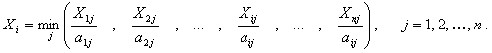
The table of intersectoral balance allows us to study the structure of resource flows, but in order to understand the functioning of the economy, in particular the effect of distribution (multiplication), we must take another step in constructing tables of direct cost coefficients and total cost coefficients.
The direct cost coefficient is defined as the amount of resource i required to produce a unit of product j, i.e., the amount of product j.
| (9-5) |
The set of cost coefficients of all sectors of the economy under consideration, presented in the form of a rectangular table corresponding to the intersectoral balance table for the same economy, is called the structural matrix of this economy. In practice, structural matrices are usually calculated on the basis of the cross-sectoral balance in value terms.
After substituting Xij = aijXj in (7-1), we get:
| (9-6) |
which brings us close to the central question of cross-industry analysis – how will the output of industry Xi change if, at a fixed coefficient of direct costs aij, the value ![]()
![]() changes to
changes to ![]() Fi , i.e. Fi =
Fi , i.e. Fi = ![]() +
+ ![]() Fi. In other words, for each industry the existence of a production function is allowed with an unchanged economies of scale (costs are directly proportional to output) and with the absence of interchangeability of resources (the ratio of costs is fixed and does not depend on the level of output).
Fi. In other words, for each industry the existence of a production function is allowed with an unchanged economies of scale (costs are directly proportional to output) and with the absence of interchangeability of resources (the ratio of costs is fixed and does not depend on the level of output).
Production functions can be written as follows:
This expression takes into account only the costs of intermediate products, the costs of factors of production are omitted. Therefore, in order to answer the question posed, we come to the need to find a solution to X1, X2, … , Xn of the system of linear equations:
| (9-7) |
To simplify the appearance of this expression, let’s resort to the matrix representation:
| X = AX + F, | (9-8) |
Where is
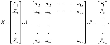
The resulting formula is the Leontief model of intersectoral balance or the linear model of intersectoral balance.
Solve the system of equations (9-8) with respect to X. We get:
X-AX=F for any finite demand vector F. Given that X=IX, where I is the unit matrix:
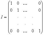
you can write:
IX-AX=(I-A)X=F
Multiplying the left and right parts of the resulting equality by the matrix (I-A)-1 (inverse of the matrix (I-A)) we have:
| X = (I – A)-1F. | (**) |
The matrix of direct cost coefficients A corresponds to the table of coefficients aij, and it is clear that not for every matrix A the system of equations (9-8) has a positive solution. It is easy to construct a matrix for which it will be impossible to pick up a pair of positive vectors X and F satisfying (9-8). For example, matrix A with elements aij>1. In this case, for any vector X>0, the inequality is executed: AX>X, therefore, AX+ F>0 at F>0 and therefore there is no X>0 that satisfies the system of equations X = AX + F.
Matrix A characterizes the economics of production, and it is natural to require that at least one set of final products can be produced. For the solution to exist, it is sufficient that the Howkins-Simon condition is satisfied, i.e. the non-negative square matrix A is productive, i.e. there is at least one vector X > 0, such that X > AH, or in the transformed form (I – A) X > 0.
G.G. Zabudsky formulates a theorem that justifies the allocation of a class of productive matrices.
Theorem: in order for the linear model of the interbranch balance X = AX + F to have a solution at any non-negative F, it is necessary and sufficient that the direct cost matrix A is productive.
There are several ways to test the productivity of matrix A: productivity criteria (necessary and sufficient conditions), as well as sufficient conditions (i.e. if they are met, then A is productive, if not, it is impossible to conclude that matrix A is unproductive).
Criteria:
Matrix A is productive if and only if there is a matrix (I-A)-1 and it is non-negative. A non-negative matrix A is productive if and only if (I-A) has n positive successive principal minors.
Sufficient conditions:
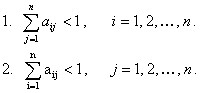
The economic meaning of the Howkins-Simon condition is as follows: an economic system in which each industry functions, directly or indirectly consuming the products of other industries, must be able to provide not only for itself, but also to make positive deliveries for final demand, and at the same time any of its subsystems must be able to do the same. If at least one of the subsystems cannot satisfy this requirement, it will inevitably cause a leak that will disrupt the ability to self-support the entire system – in mathematical economics and the theory of cross-industry models, this property is called productivity.
The matrix B=(I-A)-1 is called the inverse Leontiev matrix or, by analogy with the Keynesian concept of the multiplier, the matrix multiplier, or Leontiev multiplier. Leontiev’s inverse matrix B is, in fact, a matrix of total cost coefficients. The economic meaning of its elements bij is as follows: the coefficient bij shows the need for gross output of industry i for the production of a unit of final output of industry j. Thus, bij is essentially a multiplier showing the effect of the spread of demand, the initial source of which is the final demand for products.
It is proved that:
| I + A + A2 + … + Ak + … = (I – A)-1 | (***) |
From the expressions (**) and (***) we get:
X = (I – A)-1F = (I + A + A2 + … + Ak + …) F,
Moreover, AF is the result of the primary propagation effect, A2F – secondary, etc. From the previous ratio it follows that the solution (9-8) can be obtained iteratively (according to the Jacobi method):
| X(k+1) = AX(k) + F. | (9-9) |
Substituting in (9-9) as the initial iterative value X0 = F, we calculate the multiplication effect generated by the final demand; by setting other initial non-negative values, we will be able to evaluate the results obtained from an economic point of view.