The classical (original) Neumann model is constructed under the following premises:
An economy characterized by linear technology consists of industries, each of which has a finite number of production processes, i.e. several types of goods are produced, and joint activities of industries are allowed; production processes unfold in time, and the implementation of costs and the output of finished products are separated by a time lag; for production in this period, only those products that were produced in the previous period of time can be spent, primary factors are not involved; the population’s demand for goods and, accordingly, final consumption are not explicitly allocated; the prices of goods change over time.
Let’s move on to the description of Neumann’s model. In a discrete time interval ![]()
![]() with points
with points ![]() , production is considered, in which n types of costs are converted by means of m technological processes into n types of products. We will not specify the number of industries, since in the future it is not necessary to emphasize the belonging of goods or technologies to specific industries. In Leontiev’s model, technological coefficients were assigned to the unit of product. In Neumann’s model, taking as production units not industries, but technological processes, it is convenient to attribute these coefficients to the intensity of production processes.
, production is considered, in which n types of costs are converted by means of m technological processes into n types of products. We will not specify the number of industries, since in the future it is not necessary to emphasize the belonging of goods or technologies to specific industries. In Leontiev’s model, technological coefficients were assigned to the unit of product. In Neumann’s model, taking as production units not industries, but technological processes, it is convenient to attribute these coefficients to the intensity of production processes.
The intensity of the production process j is the volume of products produced by this process per unit of time. The level of intensity of the j-th process at time t is denoted by ![]()
![]() (
(![]() ). Note that it is a vector whose
). Note that it is a vector whose ![]() number of components corresponds to the number of types of goods
number of components corresponds to the number of types of goods ![]() and .
and .
Suppose that the operation of the j-th process (![]()
![]() ) with a unit intensity requires the expenditure of products in quantity
) with a unit intensity requires the expenditure of products in quantity
![]()
![]()
and gives the release of goods in quantity
![]()
![]()
A pair characterizes the ![]()
![]() technological potential inherent in the j-th process (its functioning with a unit intensity). Therefore, the pair
technological potential inherent in the j-th process (its functioning with a unit intensity). Therefore, the pair ![]() can be called the basis of the j-th production process, meaning that for any intensity
can be called the basis of the j-th production process, meaning that for any intensity![]() , the corresponding input-output pair can be expressed as
, the corresponding input-output pair can be expressed as ![]() . Therefore, the sequence of pairs:
. Therefore, the sequence of pairs:![]()
![]()
![]() (9-9)
(9-9)
representing the costs and outputs of all production processes in the conditions of their functioning with single intensities, we will call the basic processes.
All m basic processes are described by two matrices:
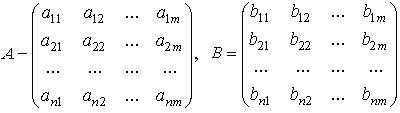 ,
,
where A is the cost matrix, B is the output matrix. The ![]()
![]() vector is called the intensity vector. The inputs and outputs corresponding to this vector for all m processes can be obtained as a linear combination of the basic processes (9-9) with the coefficients
vector is called the intensity vector. The inputs and outputs corresponding to this vector for all m processes can be obtained as a linear combination of the basic processes (9-9) with the coefficients ![]() :
:
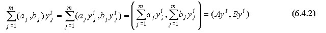 (9-10)
It is said that in the production process ![]()
![]() , the basic processes (9-9) are involved with intensity
, the basic processes (9-9) are involved with intensity ![]() . As can be seen from (9-10), Neumannian technology, described by two matrices A and B of the unit levels of input and output, is linear. Considering all the permissible “mixtures” of basic processes, we get an extended set of production processes:
. As can be seen from (9-10), Neumannian technology, described by two matrices A and B of the unit levels of input and output, is linear. Considering all the permissible “mixtures” of basic processes, we get an extended set of production processes:
![]()
![]() (9-11)
(9-11)
which reflects the permissibility of joint activities of industries. The possibility of joint production of several products in one process follows from the fact that in each process j can be more than one of the quantities ![]()
![]() different from zero. The set (9-11) is a Neumannian technology in statics (at the moment t). If you put n = m in the matrix A, the matrix B is identified with the unit matrix, and
different from zero. The set (9-11) is a Neumannian technology in statics (at the moment t). If you put n = m in the matrix A, the matrix B is identified with the unit matrix, and ![]() interpreted as a vector of gross output, then (9-10) turns into Leontief’s technology.
interpreted as a vector of gross output, then (9-10) turns into Leontief’s technology.
Let’s continue the description of neumann’s model. According to prerequisites 2) and 3), the costs ![]()
![]() at time t cannot exceed the output
at time t cannot exceed the output ![]() corresponding to the previous moment t-1 (Figure 9.1).
corresponding to the previous moment t-1 (Figure 9.1).
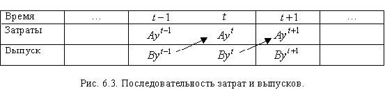
Fig.9.1.
Therefore, the following conditions must be met:
![]()
![]() (9-12)
(9-12)
where ![]()
![]() is the vector of the stock of goods by the beginning of the planned period.
is the vector of the stock of goods by the beginning of the planned period.
![]()
![]() Inequality (9-12) can be interpreted as the non-superiority of demand over supply at time t. Therefore, in value terms (in prices of the moment t) should be):
Inequality (9-12) can be interpreted as the non-superiority of demand over supply at time t. Therefore, in value terms (in prices of the moment t) should be):
![]()
![]() (9-13)
(9-13)
According to the assumption 5), the profit of the basic process ![]()
![]() on the segment [t-1,T] is equal to the value
on the segment [t-1,T] is equal to the value ![]() , i.e. costs are carried out at the price of the beginning of the period, and finished products – at the price of the moment of its sale. Thus, the costs for all basic processes can be recorded as
, i.e. costs are carried out at the price of the beginning of the period, and finished products – at the price of the moment of its sale. Thus, the costs for all basic processes can be recorded as ![]() , and revenue – as
, and revenue – as ![]() (Fig. 9.2).
(Fig. 9.2).
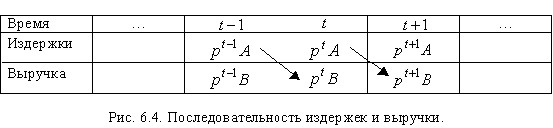
Rice. 9.2.
Let’s say that the basic processes are unprofitable if ![]()
![]() , are not profitable – if
, are not profitable – if
![]()
![]() (9-14)
(9-14)
Neumann’s model assumes the non-profitability of basic processes. This is explained by the fact that costs and revenues are diluted in time, i.e. they relate to different points in time, and in an expanding economy “a case of falling prices (![]()
![]() )” is characteristic”, i.e. the purchasing power of money at time t will be higher than at the time of t-1. One can agree or disagree with this justification. The main reason for the non-profitability of basic processes is inherent in the definition of economic equilibrium. Let us explain this in a little more detail.
)” is characteristic”, i.e. the purchasing power of money at time t will be higher than at the time of t-1. One can agree or disagree with this justification. The main reason for the non-profitability of basic processes is inherent in the definition of economic equilibrium. Let us explain this in a little more detail.
The description of the Neumann model is complete. Set of inequalities and equations
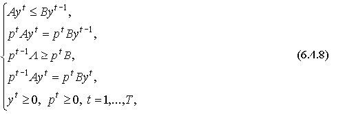 (9-15)
where ![]()
![]() and
and ![]() is the cost-output matrices, respectively, is called the (dynamic) Neumann model.
is the cost-output matrices, respectively, is called the (dynamic) Neumann model.
Definition 9.1. It is said that there is a balanced growth of production in the economy if there is such a constant number ![]()
![]() that for all m production processes:
that for all m production processes:
![]()
![]() (9-16)
(9-16)
A constant number ![]()
![]() is called the rate of balanced production growth.
is called the rate of balanced production growth.
Content (9-16) means that all intensity levels increase at the same rate

Opening the right part (9-16) recurrently, we get:
![]()
![]() (9-17)
(9-17)
where ![]()
![]() is the intensity of the process j , established by the beginning of the planning period. Note that t in the right part (9-17) is an indicator of the degree, and in the left – the index.
is the intensity of the process j , established by the beginning of the planning period. Note that t in the right part (9-17) is an indicator of the degree, and in the left – the index.
In the case of balanced production growth, taking into account the constancy of the growth rate, the sequence ![]()
![]() is called a stationary production trajectory.
is called a stationary production trajectory.
Definition 9.2. It is said that in an economy there is a balanced decline in prices if there is such a constant number ![]()
![]() that for all n goods
that for all n goods
 (9-18)
A constant number ![]()
![]() is called the rate of interest.
is called the rate of interest.
Meaningfully (9-18) means that the prices of all goods are decreasing at the same rate
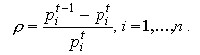
The name “rate of interest” for the rate of decline ![]()
![]() is taken by association with the indicator of the rate of interest (rate of return) in the compound interest
is taken by association with the indicator of the rate of interest (rate of return) in the compound interest ![]() formula, where R0 is the amount of the initial investment, Rn is the final amount obtained after n periods,
formula, where R0 is the amount of the initial investment, Rn is the final amount obtained after n periods, ![]() is the rate of interest.
is the rate of interest.
From equality (9-17) we get:
 (9-19)
where ![]()
![]() are the prices established at the beginning of the planning period.
are the prices established at the beginning of the planning period.
In the case of a balanced price reduction, the sequence ![]()
![]() is called a stationary price trajectory.
is called a stationary price trajectory.
Substituting (9-17) and (9-19) into the Neumann model, we get its “stationary” form:
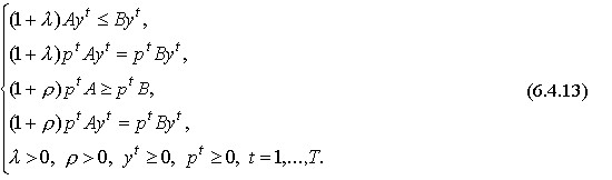 (9-20)
This system of relations shows that according to stationary trajectories y and p, the economy develops according to an unchanging dynamic law. Therefore, it is natural to call this situation equilibrium.