The problem of compensation by increasing consumer income arises in all cases where there is an increase in the prices of one or more of the goods consumed. Different approaches to solving this problem are possible. The most direct of them uses the concept of the demand function in a fairly general form and relies on the concept of compensation as such an increase in income that allows you to leave the demand for a product at the level determined by the previous price. Thus, the demand function is applied
D = D(I, p),
Where is
I – initial level of income,
p – initial price level.
Let’s designate a new price level:
![]()
![]() ,
,
a compensating change in income
![]()
![]() .
.
It is easy to see that demand remains unchanged if a condition is met.
 .
.
For normal and valuable goods ![]()
![]() and , therefore
and , therefore ![]() , with an increase in price (Δp>0), an increase in income in the amount of
, with an increase in price (Δp>0), an increase in income in the amount of
 .
.
In the specific case where the demand function is:
![]()
![]() ,
,
we get the following simple relationship between price increase and compensation
 or
or  .
.
This means that the relative increase in income must be proportional to the relative change in price with a proportionality coefficient equal to the ratio of elasticities of these factors.
In the more complex case of many goods, this approach is based on the use of demand functions of the form:
![]()
![]()
An increase in the price of one of the goods (for example, with the number n) changes, generally speaking, the demand for each product. If there is a ratio for some product j:
 ,
,
i.e. when the price of good n rises, the demand for good j falls, then products n and j are complementary (e.g. cars and gasoline).
It is not difficult to see that if there are complementary ones among the list of goods, then in the general case it is impossible to accurately solve the problem of compensation by increasing income.
If the inequality is true for the product j:
 ,
,
i.e. an increase in the price of the commodity “n” causes an increase in demand for the product “j”, then they are called interchangeable (butter and margarine). The demand function has the property of strong gross fungibility if all goods are interchangeable. It is not difficult to see that in this case, an increase in the price of one product leads to a decrease in demand only for this product, but increases the demand for all the others. In this situation, the approach discussed above for the case of a single product can be used to calculate the necessary compensation. However, this results in too high a level of compensation, since the consumption of almost all goods will increase.
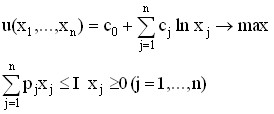
In this regard, a more economical way of estimating the amount of compensation, based on the use of the concept of a utility function, is used. With this approach, the volume of demand for various goods is considered as a solution to the problem of the optimal choice of the consumer in conditions of limited income:
u(x1, …, xn) → max

xj ≥ 0 (j = 1, …, n)
The solution to this problem:
![]()
![]()
determines the maximum achievable level of the utility ![]()
![]() function, which obviously depends on both the price system p = (p1, …, pn) and the income level I.
function, which obviously depends on both the price system p = (p1, …, pn) and the income level I.
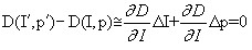
Let now, as before, increase the price of pn of the commodity “n”. The solution to the modified problem will be such that the maximum level ![]()
![]() will decrease. In this regard, a natural question arises: how much income I needs to be increased in order to restore the previous value
will decrease. In this regard, a natural question arises: how much income I needs to be increased in order to restore the previous value ![]() of , and consequently, the previous level of consumer satisfaction. In a fairly general form, the answer to this question is given by the Slutsky equation, the main conclusions from which will be further considered on a simple example.
of , and consequently, the previous level of consumer satisfaction. In a fairly general form, the answer to this question is given by the Slutsky equation, the main conclusions from which will be further considered on a simple example.
Let n=2, the utility function:
![]()
![]() .
.
The solution to the problem of optimal choice is:
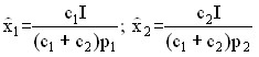 .
.
Maximum level of utility function:
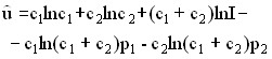
The condition for maintaining the maximum level is as follows:
![]()
![]() or
or 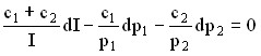 .
.
From here we get an expression for compensation in case of price changes:
![]()
![]() .
.
Thus, if the price of p2 increases (dp2 > 0) and the price of p1 remains unchanged (dp1 = 0), then the demand for the second product will fall, and the demand for the first product will not change. The amount of compensation is determined in this case by the ratio
![]()
![]()
Thus, the achieved level of satisfaction will be maintained if the income is increased just enough so that the consumer can purchase the previous volume of the second product. However, it is not difficult to show that in fact the consumer uses compensation as follows: his demand for a product with an increased price (product 2) will decrease, but the volume of purchases of the first product will increase. At the same time, the level of utility will remain the same as it was before the price increases and compensation was received. An illustration of this transition can be found in Figure 5.19.
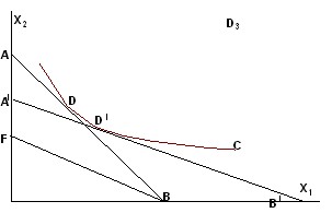
Rice. 5.19. Optimal set in case of price changes and compensation
In here:
line C – the indifference curve corresponding to the maximum level of utility; line AB – budget line before price increases; point D – optimal set; FB line – budget line after the price increase p2, but before compensation is paid; line A′B′ – budget line after payment of compensation (A′B′ || FB), point D′ is the optimal set in the new conditions.
In the more general case, when the problem of optimal choice is:
 ,
,
it can be shown that the compensation surcharge, which maintains the same level of maximum utility, is associated with a change in prices by the ratio:
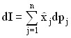 ,
,
where ![]()
![]() is the optimal demand for j – the product before the price changes, and
is the optimal demand for j – the product before the price changes, and ![]() – the change in the price of the j-th product.
– the change in the price of the j-th product.