The basis for the study of personal consumption (individual consumers and households) are indifference curves. The indifference curve is a line, each point of which represents such a combination of two goods that the consumer does not care which of them to choose. Indifference curves graphically reflect the consumer’s system of preferences.
For the convenience of reproduction, a two-dimensional space is used, because the conclusions obtained for the two-dimensional case (for two goods) are valid for an arbitrarily large number of goods.
Let’s look at a simple example. Suppose a household can consume two kinds of goods (good 1 and good 2). Let for some period the first good be consumed in the amount of y1, and the second in the amount of Y2. The two-dimensional vector (y1, y2) is called the consumption plan. The household compares the vector of consumption (the set of consumed goods) A = (Y1A, Y2A) with another vector of consumption, B = (Y1B, Y2B) and makes one of the following judgments:
(a) Vector A is preferable to vector B;
b) vector B is preferable to vector A;
c) vectors A and B are equally preferred (the consumer does not care which of the vectors A or B to choose).
The indifference curve here is all consumption plans that are in a relationship of indifference with the consumption plan in question.
If we denote through U = U(y1, y2) a function, or in other words, an index of utility that can be obtained from the consumption of goods specified by the vector (y1, y2), then the indifference curve is a set of values.
(y1, y2), which result in the same U value.
There are different kinds of indifference curves defined by the way a utility function is set. But there are also general properties of the indifference curve, regardless of its type:
it is always possible to draw a corresponding indifference curve through any point in the graphic space of goods, because for any combination of two goods there will always be many other combinations, the usefulness of which will be the same as that of this point. This property is based on the fact that the consumer can compare all goods or their set using relations of preference or indifference (the axiom of complete orderliness); indifference curves never intersect (transitivity axiom and unsaturation axiom); Based on the first two properties, you can build a map of indifference curves containing information about the consumer preference system. A curve more distant from the origin has a greater overall utility: preferable; the indifference curve has a negative slope, since the reduction in the quantity of one good must be compensated or replaced by an increase in the quantity of another good in order to preserve the overall utility of the set; the indifference curve in the broad sense is concave with respect to the origin: the slope of the indifference curve decreases when moving along the horizontal axis from the origin. This is explained by the fact that the consumer’s willingness to replace one product with another falls.
To construct an indifference curve, it is necessary to express one of the arguments of the utility function through another argument and the value of the utility function U. Thus, for the utility function (1), we get:
 ,
,
and for function (2) we get:
 .
.
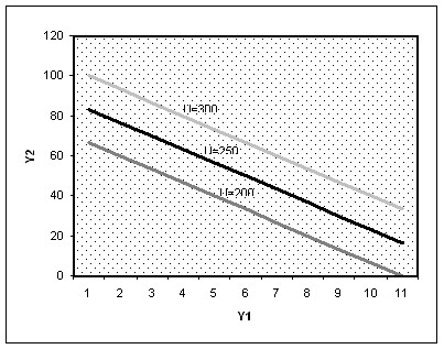
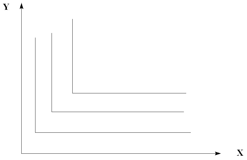
Rice. 5.7. Indifference Curves
This type of curve (Fig. 5.7.) is inherent in substitute goods, and absolute ones at that. This means that an increase in demand for one of the two goods (goods) is accompanied by a drop in demand for the other good: these two goods are in a relationship of interchangeability. Examples include coffee and tea.
Regarding the last property of the indifference curve, when replacing the strict inequality with a non-strict in the condition of concavity of the function, we come to the concept of a concave linear function.
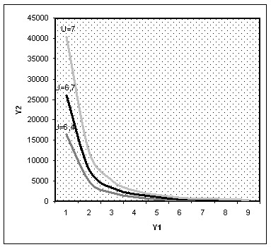
Fig.5.8. Indifference curves
The type of these curves (Fig. 5.8.), strictly speaking, is one of the mixed, since there is also a type of indifference curves for complementary goods (goods). As the demand for one of these two goods increases, so does the demand for the second good: they are in a complementary relationship. For example, coffee and sugar.
Consider sets of only two goods Χ and Υ. (Goods Χ and Υ can be considered as combined goods).
The preference relations characteristic of each individual are reflected by means of an indifference curve (Fig. 5.9.).
The indifference curve reflects a set of points, each of which is such a set of two goods that the consumer does not care which of these sets to choose. Sets A and B are equivalent in terms of this consumption and lie on the same indifference curve. For our consumer, any set lying on curve II is preferable to any set lying on curve I, etc.
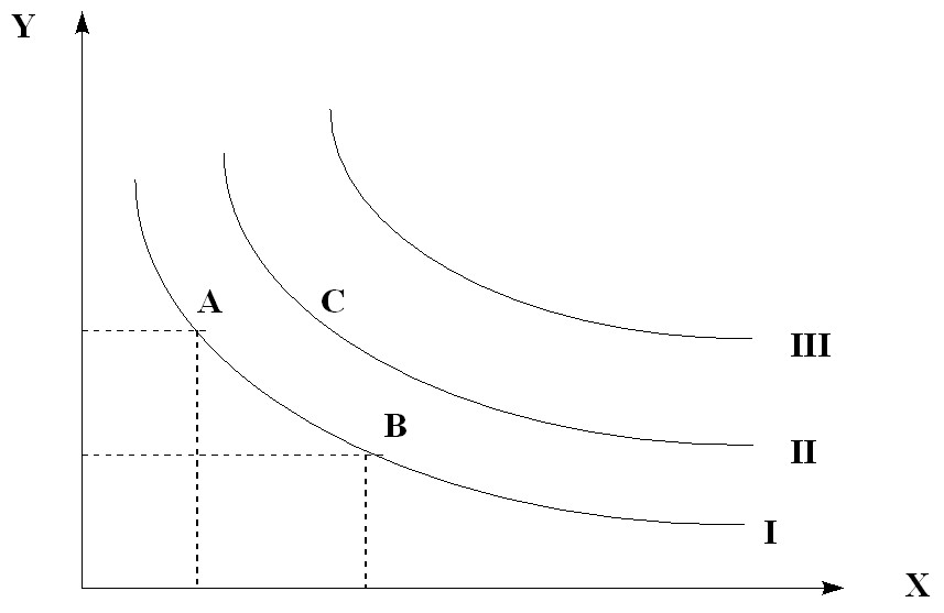
Rice. 5.9. Indifference Curves
Depending on the utility functions, the following types of indifference curves are distinguished:
1). The utility function with full substitution of goods (tea and coffee) has the form:
![]()
![]() ,
,
where a,b are the parameters;
U – utility;
X,Y – goods.
From the utility function you can find Y:

![]()
and to construct indifference curves of linear type (Fig. 5.10.).
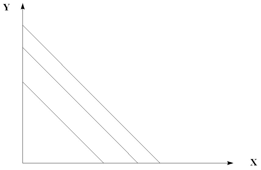
Rice. 5.10. Linear type indifference curves
2). The neoclassical utility function is:
![]()
![]() where a+b ≤ 1
where a+b ≤ 1
To construct indifference curves, you need to find Y:

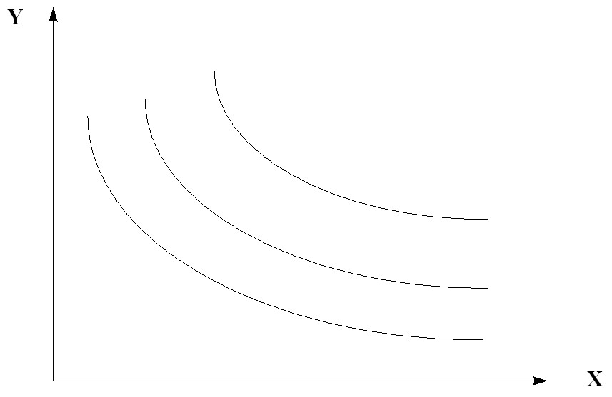
Rice. 5.11. Curves of indifference of the neoclassical type
3) Functions with a complete complementarity of goods (with an increase in demand for one of the two goods, the demand for the second good, for example, sugar and tea, gasoline and motor oil) have indifference curves in the form of a point at the intersection of two straight lines. The excess of one good does not matter. Utility is achieved only with a certain combination of both goods.
Rice. 5.12. Indifference curves of functions with complete complementarity of goods
The basic concepts of consumption theory are marginal utility and marginal replacement rate. Let U(Y1, Y2) be a utility function. The increase in the utility function achieved at a fixed level of consumption of the first good and a slight change in the level of consumption of the second good is called the marginal utility of the second good. That is, marginal utility is the utility derived from the consumption of an additional unit of good.
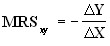
The value that determines the slope of the indifference curve is called the marginal rate of substitution; MRS) consumer goods. It shows the extent to which the consumer is willing to replace one product with another in order to obtain the same overall utility.
In other words, the marginal rate of substitution of good X of the good Y (MRSxy) is the amount of good Y that must be reduced “in exchange” for an increase in the quantity of good X by one, so that the level of satisfaction of the consumer remains unchanged:
 provided that U= const
According to the axiom of unsaturation, any point lying above the indifference curve is always preferable to the consumer, possessing greater overall utility. And any point below the indifference curve is correspondingly less preferable to the consumer.
If we use the utility function of the neoclassical type, we can see the existence of the law of the decreasing marginal rate of substitution. This law was the result of the interpretation of the law of diminishing marginal utility from the standpoint of the theory of choice (the theory of ordinal utility, the ordinalist approach) and is considered one of the central ideas of modern microeconomic theory. The law of the decreasing marginal rate of substitution can be formulated as follows: when striving to maintain an unchanged level of utility by replacing the first good with the second, the subjective satisfaction obtained from the marginal consumption of the first good, in comparison with the satisfaction obtained from the marginal consumption of the second good, will steadily decrease.
Naturally, the consumer seeks to purchase a commodity set belonging to the indifference curve furthest from the origin. However, this is not always possible, because consumer behavior is limited by the means at his disposal.
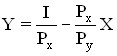
If we denote the market prices of the good X through Px, and the goods Y through Py,![]()
![]() and its income through I, then the budget constraint of the consumer can be written in the form of an equation:
and its income through I, then the budget constraint of the consumer can be written in the form of an equation:
![]()
![]() .
.
The consumer’s income is equal to the sum of his expenses for the purchase of goods X and Y.
Transform the equation and get the equation of the budget line, which has the form of a straight line (Fig. 5.13.). The higher the income, the farther from the origin of the coordinates is the line of the budget limit.
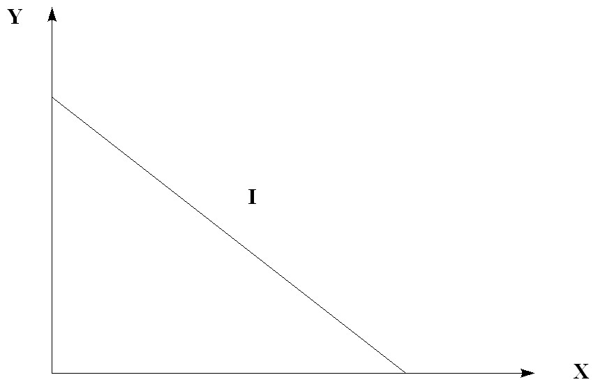
Rice. 5.13. Budget line
Let be a budget constraint line and a few indifference curves. What product set does the consumer choose?
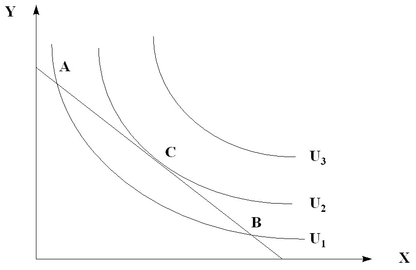
Rice. 5.14. Optimal consumer choice
The consumer’s optimum will be at point C. Within the budget constraint, the individual will try to distribute his income among different goods in such a way as to maximize the utility of U. The corresponding set of goods is called the optimal consumption plan and is usually indicated by the point of contact of the budget line and the indifference curve. So, in conditions when the market prices and income of the individual are set from the outside, the optimal plan of consumption of the individual is determined on the basis of the principle of maximizing utility. The optimal consumption plan varies depending on prices and income (Figure 5.14.).
At the optimum point, the equality is:

The ratio of the price of the good X to the price of the good Y is equal to the marginal rate of substitution of the good X of the good Y.
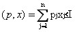
In general, consider a consumer (a group of families) with a certain income I, intended for the purchase of a set of goods X = (x1 ,…, xj ,…, xn), the prices of which are respectively equal to P = (p1 ,…, pj ,…, pn).
Here X,P are non-negative vectors.
The limited choice of the consumer is expressed by means of a budget constraint
The formulation of the problem of optimal consumer choice can be formulated in two ways: a) in terms of the preference ratio: the best (optimal) is the set ![]()
![]() , which is “the most preferable in relation to ” =
, which is “the most preferable in relation to ” =![]() ” among all non-negative x vectors satisfying the budget constraint. The most preferred set on a set R is usually a set
” among all non-negative x vectors satisfying the budget constraint. The most preferred set on a set R is usually a set![]() having the property that it satisfies the condition
having the property that it satisfies the condition
“![]()
![]() =
=![]() x” for all x ∈ R
x” for all x ∈ R
Obviously, the uniqueness of such a set, generally speaking, is not ensured.
b) in terms of the utility function: the optimal set ![]()
![]() corresponds to the highest value of u(x) under the above conditions, i.e. is a solution to the problem:
corresponds to the highest value of u(x) under the above conditions, i.e. is a solution to the problem:
u(x) = u(x1 ,…, xj ,…, xn) → max
under conditions
 ; xj ≥ 0 (j = 1, … , n)
When analyzing the problem of optimal choice, another important assumption of consumption theory is usually applied, which is called the consumer’s unsaturation hypothesis and consists in the fact that for any two sets x and y the ratio is valid:
if x ≥ y, then “x =![]()
![]() y”.
y”.
A more accurate ratio is also considered fair:
if x ≥ y and x ≠ y, then “x > y”.
This means that for the “unsaturated” consumer, any set of x that contains any product as much, or (at least one item) slightly more than set y, is more preferable. The assumption of unsaturation using the utility function is expressed as follows:
if x ≥ y, then u(x) ≥ u(y). if x ≥ y and x ≠ y, then u(x) > u(y).
Thus, the utility function is monotonously increasing for each argument xj .
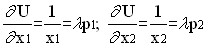
If the utility function has derivatives in its arguments, then it follows from the assumption of insatiability (and monotony u(x)) that all the first partial derivatives of the utility function are positive, i.e.:
 (j = 1, …, n)
for any set of consumer goods. The value of the partial derivative:

it makes the following economic sense: it shows how much the utility of the set will increase if the amount of good consumed increases by a “small unit”. In this regard, this derivative is called marginal (marginal, differential) utility.
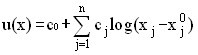
In economic studies, as a rule, some specific types of convex utility functions are used, and the selection of the type of function and the assessment of numerical values of parameters are made on the basis of observations and analysis of consumer behavior. The most commonly used linear, quadratic and logarithmic functions of the form are:
In the space of two-element sets of x=(x1, x2), the indifference surface (i.e., the lines u(x1, x2)=const) are usually called indifference curves.
For example, for a logarithmic function:
u(x1, x2)= log x1 + log x2
the indifference curves are as follows:
log x1 + log x2 = log (x1 x2) = const ,
i.e. are simply hyperbolas in the positive ortant satisfying the equations:
(x1 ⋅ x2) = const
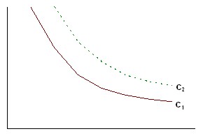
Rice. 5.15. Indifference Curves
In Fig. 5.15 C2 > C1, i.e. a higher indifference curve corresponds to a greater level of utility of those sets that make up the indifference curve.
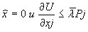
Consider the problem of the optimal choice of the consumer for the unsaturated consumer:
It is easy to see that the optimal set ![]()
![]() (
(![]() ,
,![]() ,
, ![]() ) must satisfy the budget constraint as an exact equality. Indeed, if the optimal set were to be achieved provided that:
) must satisfy the budget constraint as an exact equality. Indeed, if the optimal set were to be achieved provided that:
 ,
,
then the consumer could buy with the remaining money a certain amount of any good, and thereby get a new set with greater utility. This means that the inner point of a set cannot be an optimal set.
Thus, the problem of the optimal set is:
u(x) = u(x1 ,…, xj ,…, xn) → max
 .
.
The solution to this problem on a conditional extremum is using the method of multipliers. The optimal set is determined by solving the following system from the (n+1) equation:
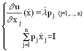
with respect to (n+1)-th unknown, namely the elements of the optimal set (![]()
![]() , ,
, ,![]()
![]() ) and the Lagrange
) and the Lagrange ![]() multiplier .
multiplier .
Thus, with a given system of prices, the consumer must choose such a set, and for which all marginal utilities are proportional to prices. At the same time, the optimal value of the Lagrangian ![]()
![]() multiplier is often called the “marginal utility of money” and is interpreted as an increase in maximum utility with an increase in income I by a small unit. Note that the optimality ratios can be represented in the form of:
multiplier is often called the “marginal utility of money” and is interpreted as an increase in maximum utility with an increase in income I by a small unit. Note that the optimality ratios can be represented in the form of:
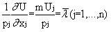 ,
,
which allows for a curious interpretation: at the optimal point, the amount of additional utility per monetary unit should be the same for all goods and services. It should also be noted that for some goods the following ratios can be performed:
 ,
,
which mean that such goods are comparatively of little use and relatively expensive, and therefore should not be included in the optimal set of consumers maximizing their utility with limited income.
Let’s look at a simple example.
Let n=2, the utility function:
u(x1, x2) = ln x1 + ln x2,
budget limit:
p1x1 + p2x2 = I.
Solving the problem of optimal choice
hence:
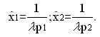
Using the budget limit, we have:
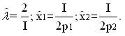
As can be seen from the above solution, the optimal choice of the consumer has a very natural form: the amount of goods consumed is directly proportional to income (I) and inversely proportional to its price. The geometric interpretation of the solution of the problem of optimal choice is shown in Fig. 5.14.
In more realistic options for setting the problem of optimal choice with the help of additional conditions, restrictions on the range of goods and services consumed, the possibility of mutual replacement of various products, etc. can be taken into account.