To solve the problems of economic analysis and forecasting, statistical, reporting or observable data are very often used. At the same time, it is believed that these data are values of a random variable.
A random variable is a variable that, depending on the case, takes different values with some probability. The law of distribution of a random variable shows the frequency of its certain values in their totality.
When studying the relationships between economic indicators based on statistical data, there is often a stochastic relationship between them. It is manifested in the fact that a change in the law of distribution of one random variable occurs under the influence of a change in another. The relationship between quantities can be complete (functional) and incomplete (distorted by other factors).
An example of functional dependence is the output of products and its consumption in conditions of scarcity.
An incomplete relationship is observed, for example, between the length of service of workers and their labor productivity. Usually, workers with a long work experience work better than young ones, but under the influence of additional factors – education, health, etc. This dependence can be distorted.
The section of mathematical statistics devoted to the study of relationships between random variables is called correlation analysis. The main task of correlation analysis is to establish the nature and closeness of the relationship between effective (dependent) and factor (independent) indicators (signs) in a given phenomenon or process. Correlation can be detected only by mass comparison of facts.
The nature of the relationship between the indicators is determined by the correlation field. If Y is a dependent feature and X is an independent feature, then by ticking each case of X(i) with coordinates xi and yi, we get a correlation field.
The closeness of the connection is determined using the correlation coefficient, which is calculated in a special way and lies in the intervals from minus one to plus units. If the value of the correlation coefficient lies in the range from 1 to 0.9 modulo, then there is a very strong correlation relationship. If the value of the correlation coefficient lies in the range from 0.9 to 0.6, then it is said that there is a weak correlation. Finally, if the value of the correlation coefficient is in the range from -0.6 to 0.6, then they speak of a very weak correlation dependence or its complete absence.
Thus, correlation analysis is used to find the nature and closeness of the relationship between random variables.
Regression analysis is aimed at deriving, defining (identifying) the regression equation, including statistical estimation of its parameters. The regression equation allows you to find the value of a dependent variable if the value of the independent or independent variables is known.
In practice, it is a question of analyzing the set of points on the chart (i.e. a set of statistical data), finding a line that, if possible, accurately reflects the pattern (trend, trend) contained in this set – the regression line.
According to the number of factors, one-, two- and multifactorial regression equations are distinguished.
According to the nature of the relationship, one-factor regression equations are divided into:
(a) Linear:
![]()
![]()
![]() ,
,
where X is an exogenous (independent) variable;
Y – endogenous (dependent, effective) variable;
a, b – parameters.
b) power:
![]()
![]()
![]()
c) illustrative:
![]()
![]()
d) other.
Determination of the parameters of the linear one-factor regression equation
Suppose we have data on income (X) and demand for some commodity (Y) for a number of years (n)
YEAR n | INCOME X | DEMAND Y |
1 | x1 | y1 |
2 | x2 | y2 |
3 | x3 | y3 |
… | … | … |
n | xn | yn |
Suppose that there is a linear relationship between X and Y, i.e., a linear relationship between X and Y.
![]()
![]()
In order to find the regression equation, first of all it is necessary to investigate the closeness of the relationship between the random variables X and Y, i.e. the correlation relationship.
Let:
x![]()
![]() , x
, x![]() , . . . , xn – the set of values of an independent, factorial feature;
, . . . , xn – the set of values of an independent, factorial feature;
y![]()
![]() , y
, y![]() . . . , yn is a set of corresponding values of the dependent, effective feature;
. . . , yn is a set of corresponding values of the dependent, effective feature;
n is the number of observations.
To find the regression equation, the following values are calculated:
Averages
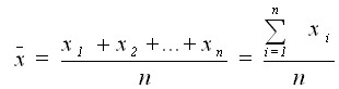 for an exogenous variable.
 for endogenous variable$
2. Deviations from the average values
![]()
![]() ,
, 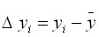 $
$
Variance and mean squared deviation
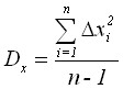 ,
, 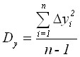 .
.

![]()
The values of variance and mean quadratic deviation characterize the spread of observed values around the average value. The greater the variance, the greater the spread.
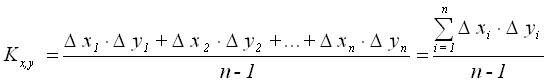
Calculation of the correlation moment (covariance coefficient):
The correlation moment reflects the nature of the relationship between x and y. If ![]()
![]() , then the relationship is direct. If
, then the relationship is direct. If ![]() , then the relationship is inverse.
, then the relationship is inverse.
The correlation coefficient is calculated by the formula:
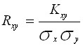 .
.
It has been proved that the correlation coefficient is in the range from minus one to plus one (![]()
![]() ). The correlation coefficient squared (
). The correlation coefficient squared (![]() ) is called the coefficient of determination.
) is called the coefficient of determination.
If ![]()
![]() , then the calculations continue.
, then the calculations continue.
Calculations of the parameters of the regression equation.
Coefficient b is found by the formula:

After that, you can easily find the parameter a:
![]()
![]()
The coefficients a and b are the method of least squares, the main idea of which is that the sum of the squares of the difference (residues) between the actual values of the resulting feature ![]()
![]() and its calculated values
and its calculated values ![]() obtained using the regression equation is taken as a measure of the total error.
obtained using the regression equation is taken as a measure of the total error.
![]()
![]() .
.
In this case, the values of the residues are found according to the formula:
![]()
![]() , where
, where
![]()
![]() The actual value of y
The actual value of y
![]()
![]() the estimated value of y.
the estimated value of y.
Example. Suppose we have statistics on income (X) and demand (Y). It is necessary to find a correlation between them and determine the parameters of the regression equation.
YEAR n | INCOME X | DEMAND Y |
1 | 10 | 6 |
2 | 12 | 8 |
3 | 14 | 8 |
4 | 16 | 10,3 |
5 | 18 | 10,5 |
6 | 20 | 13 |
Suppose that there is a linear relationship between our quantities.
Then the calculations are best done in Excel using statistical functions;
AVERAGE – to calculate average values;
VARP – to find variance;
STDEV – to determine the mean square deviation;
CORELL – to calculate the correlation coefficient.
The correlation moment can be calculated by finding deviations from the average values for the series X and series Y, then using the SUMPROIZ function to determine the sum of their products, which must be divided by n-1.
The results of the calculations can be summarized in a table.
Parameters of the linear single-factor regression equation
Indicators | X | Y |
Medium | 15 | 9,3 |
Dispersion | 14 | 6,08 |
Average quadr. deviation | 3,7417 | 2,4658 |
Correlation moment | 8,96 | |
Correlation coefficient | 0,9712 | |
Options | b=0,64 | a = – 0,3 |
As a result, our equation will be:
y = – 0.3 + 0.64x
Using this equation, you can find the estimated values of Y and plot (Figure 2.1).
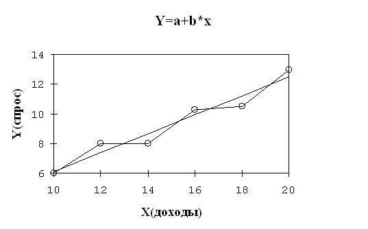
Rice. 2.1. Actual and calculated values ![]()
![]()
The broken line on the chart reflects the actual Y values, and the straight line is constructed using the regression equation and reflects the trend of change in demand depending on income.
However, the question arises, how significant are parameters a and b? What is the margin of error?
Estimation of the error value of a linear single-factor equation
Let’s denote the difference between the actual value of the effective feature and its calculated value as ![]()
![]() :
:
![]()
![]() , where
, where
![]()
![]() The actual value of y
The actual value of y
![]()
![]() calculated value y,
calculated value y,
![]()
![]() is the difference between the two.
is the difference between the two.
As a measure of the total error, the following value is chosen:
 .
.
For our example , S = 0.432.
Since ![]()
![]() (the average value of the residues) is zero, the total error is equal to the residual variance:
(the average value of the residues) is zero, the total error is equal to the residual variance:
The residual variance is found according to the formula:
![]()
![]()
For our example![]()
![]() , we can show that
, we can show that
![]()
![]() .
.
If ![]()
![]()
![]() then
then ![]()
![]()
![]() that
that ![]()
Thus, ![]()
![]() .
.
It is easy to see that if ![]()
![]() , then
, then
![]()
![]()
This ratio shows that in economic applications, the permissible total error can be no more than 20% of the variance of the resulting feature ![]()
![]() .
.
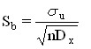
The standard error of the equation is found in the formula:
![]()
![]() Where is
Where is
![]()
![]() – residual dispersion. In our case
– residual dispersion. In our case ![]() , .
, .
The relative error of the regression equation is calculated as:
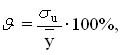
where ![]()
![]() is the standard error;
is the standard error;
![]()
![]() is the average value of the resulting feature.
is the average value of the resulting feature.
In our case ![]()
![]() , = 7.07%.
, = 7.07%.
If the value is ![]()
![]() small and there is no autocorrelation of residues, then the predictive qualities of the estimated regression equation are high.
small and there is no autocorrelation of residues, then the predictive qualities of the estimated regression equation are high.
The standard error of the coefficient b is calculated by the formula:
In our case, it is equal to ![]()
![]() .
.
To calculate the standard error of the coefficient a, the formula is used:
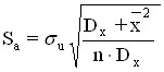
In our example ![]()
![]() , .
, .
Standard coefficient errors are used to estimate the parameters of the regression equation.
Coefficients are considered significant if
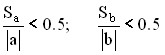
In our example 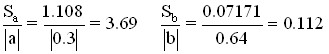
The coefficient is not significant, because this ratio is greater than 0.5, and the relative error of the regression equation is too high – 26.7%.
Standard coefficient errors are also used to estimate the statistical significance of coefficients using student’s criterion t. The values of the Student’s criterion t are found in reference books on mathematical statistics. Table 2.1 shows some of its values.
The following are the maximum and minimum values of the parameters (![]()
![]() ) according to the formulas:
) according to the formulas:
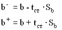
Table 2.1 Resource requirements by component
Some values of t – Student’s criterion
Degrees of freedom | Trust level (c) | |
(n-2) | 0,90 | 0,95 |
1 | 6,31 | 12,71 |
2 | 2,92 | 4,30 |
3 | 2,35 | 3,18 |
4 | 2,13 | 2,78 |
5 | 2,02 | 2,57 |
For our example we find:
![]()
![]()
![]()
![]()
![]()
![]()
If the interval (![]()
![]() ) is small enough and does not contain zero, then the coefficient b is statistically significant at the c-percentage confidence level.
) is small enough and does not contain zero, then the coefficient b is statistically significant at the c-percentage confidence level.
Similarly, there are maximum and minimum values of parameter a. For our example:
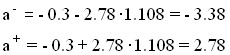
Coefficient a is not statistically significant because the interval (![]()
![]() ) is large and contains zero.
) is large and contains zero.
Conclusion: the results obtained are not significant and cannot be used for forecast calculations. The situation can be corrected in the following ways:
(a) Increase the number of n;
b) increase the number of factors;
c) change the shape of the equation.
The problem of autocorrelation of residues. Darbin-Watson criterion
Often, time series are used to find regression equations, i.e. a sequence of economic indicators for a number of years (quarters, months) following each other.
In this case, there is some dependence of the subsequent value of the indicator, on its previous value, which is called autocorrelation. In some cases, this kind of dependence is very strong and affects the accuracy of the regression coefficient.
Let the regression equation be constructed and have the form:
![]()
![]()
![]()
![]() is the error of the regression equation in year t.
is the error of the regression equation in year t.
The phenomenon of autocorrelation of residues is that in any year t the residue ![]()
![]() is not a random variable, but depends on the size of the remnant of the previous year
is not a random variable, but depends on the size of the remnant of the previous year ![]() .
.
To determine the presence or absence of autocorrelation, the Darbin-Watson criterion is applied:
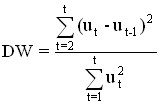 .
.
The possible values of the DW criterion range from 0 to 4. If there is no autocorrelation of residues, then DW≈2.
Construction of the power regression equation
The equation of power aggression is:
![]()
![]() Where is
Where is
a, b – parameters that are determined from the data of the observation table.
The table of observations is compiled and has the form:
x | x1 | x2 | … | xn |
y | y1 | y2 | … | yn |
Prologarithm the original equation and as a result we get:
![]()
![]() ln y = ln a + b⋅ln x .
ln y = ln a + b⋅ln x .
Denote ln y with ![]()
![]() , ln a as
, ln a as ![]() , and ln x as
, and ln x as ![]() .
.
As a result of substitution, we get:
![]()
![]()
This equation is nothing more than a linear regression equation, the parameters of which we are able to find.
To do this, let’s prologarithm the initial data:
ln x | ln x1 | ln x2 | … | ln xn |
ln y | ln y1 | ln y2 | … | ln yn |
Next, it is necessary to perform the known computational procedures for finding the coefficients a and b, using the prologarithmated initial data. As a result, we get the value of the coefficient b and ![]()
![]() . The parameter a can be found by the formula:
. The parameter a can be found by the formula:
![]()
![]() .
.
For the same purpose, you can use the EXP function in Excel.
Two-factor and multifactor regression equations
The linear two-factor regression equation is:
![]()
![]() ,
,
where ![]()
![]() are the parameters;
are the parameters;
![]()
![]() – exogenous variables;
– exogenous variables;
y is an endogenous variable.
Identifying this equation is best done by using the Excel LINEST function.
The power two-factor regression equation is:
![]()
![]()
where ![]()
![]() are the parameters;
are the parameters;
![]()
![]() – exogenous variables;
– exogenous variables;
Y is an endogenous variable.
To find the parameters of this equation, it is necessary to prologarithm it. As a result, we get:
![]()
![]()
![]() .
.
Identifying this equation is also best done by using the Excel LINEST function. It should be remembered that we will not get the parameter a, but its logarithm, which should be converted to a natural number.
The linear multifactorial regression equation is:
![]()
![]()
where ![]()
![]() n are the parameters;
n are the parameters;
![]()
![]() n – exogenous variables;
n – exogenous variables;
y is an endogenous variable.
Identifying this equation is also best done by using the Excel LINEST function.