After the regression equation is constructed and its accuracy is estimated using the coefficient of determination, the question remains how this accuracy is achieved and, accordingly, whether this equation can be trusted. The fact is that the regression equation was built not on the general population, which is unknown, but on a sample from it. Points from the general population fall into the sample randomly, so in accordance with the theory of probability, among other cases, it is possible that the sample from the “broad” general population will be “narrow” (Fig. 15).
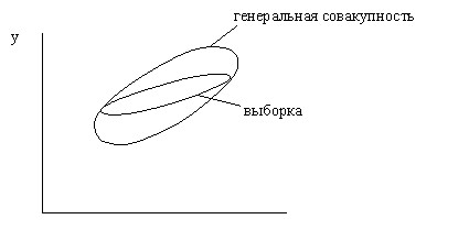
Rice. 15. A possible option for points to get into the sample from the general population.
In this case:
(a) The sample regression equation may differ significantly from the regression equation for the population, resulting in prediction errors;
b) the coefficient of determination and other accuracy characteristics are unreasonably high and misleading about the predictive qualities of the equation.
In the extreme case, the option is not excluded when a sample will be obtained from the general population of which is a cloud with the main axis of a parallel horizontal axis (there is no connection between the variables) due to random selection, the main axis of which will be inclined to the axis. Thus, attempts to predict the next values of the general population based on the sample data from it are fraught not only with errors in assessing the strength and direction of the relationship between the dependent and independent variables, but also with the danger of finding a connection between variables where in fact there is none.
In the absence of information about all points of the general population, the only way to reduce errors in the first case is to use the regression equation method when evaluating the coefficients of the regression equation, which ensures their non-displacement and efficiency. And the probability of occurrence of the second case can be significantly reduced due to the fact that a priori one property of the general population with two variables independent of each other is known – it does not have this connection. This reduction is achieved by checking the statistical significance of the resulting regression equation.
One of the most commonly used validation options is as follows: For the resulting regression equation, -statistics is defined ![]()
![]() – a characteristic of the accuracy of the regression equation, which is the ratio of that part of the variance of the dependent variable that is explained by the regression equation to the unexplained (residual) part of the variance. The equation for determining
– a characteristic of the accuracy of the regression equation, which is the ratio of that part of the variance of the dependent variable that is explained by the regression equation to the unexplained (residual) part of the variance. The equation for determining ![]() -statistics in the case of multivariate regression is:
-statistics in the case of multivariate regression is:
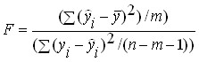
where:  – explained variance is the part of the variance of the dependent variable Y which is explained by the regression equation;
 – residual variance – the part of the variance of the dependent variable Y which is not explained by the regression equation, its presence is a consequence of the action of the random component;
![]()
![]() – the number of points in the sample;
– the number of points in the sample;
![]()
![]() is the number of variables in the regression equation.
is the number of variables in the regression equation.
As can be seen from the above formula, variances are defined as the quotient of dividing the corresponding sum of squares by the number of degrees of freedom. The number of degrees of freedom is the minimum required number of values of the dependent variable, which are sufficient to obtain the desired characteristic of the sample and which can vary freely, taking into account that all other values used to calculate the desired characteristic are known for this sample.
To obtain residual variance, the coefficients of the regression equation are necessary. In the case of paired linear regression, there are two coefficients, therefore, according to the formula (taking ![]()
![]() ) the number of degrees of freedom is
) the number of degrees of freedom is ![]() . It is understood that in order to determine the residual variance, it is sufficient to know the coefficients of the regression equation and only the
. It is understood that in order to determine the residual variance, it is sufficient to know the coefficients of the regression equation and only the ![]() values of the dependent variable from the sample. The remaining two values can be calculated on the basis of these data, and therefore are not freely variable.
values of the dependent variable from the sample. The remaining two values can be calculated on the basis of these data, and therefore are not freely variable.
To calculate the explained variance of the values of the dependent variable, it is not required at all, since it can be calculated by knowing the regression coefficients for the independent variables and the variance of the independent variable. In order to verify this, it is enough to recall the expression given earlier ![]()
![]() . Therefore, the number of degrees of freedom for residual variance is equal to the number of independent variables in the regression equation (for paired linear regression
. Therefore, the number of degrees of freedom for residual variance is equal to the number of independent variables in the regression equation (for paired linear regression ![]() ).
).
As a result ![]()
![]() , the -criterion for the paired linear regression equation is determined by the formula:
, the -criterion for the paired linear regression equation is determined by the formula:
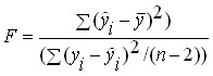 .
.
In probability theory, it is proved that ![]()
![]() the -criterion of the regression equation obtained for a sample from a general population in which there is no relationship between the dependent and the independent variable has a Fisher distribution that is well understood. Thanks to this, for any value
the -criterion of the regression equation obtained for a sample from a general population in which there is no relationship between the dependent and the independent variable has a Fisher distribution that is well understood. Thanks to this, for any value ![]() of the -criterion, it is possible to calculate the probability of its occurrence and vice versa, to determine the value
of the -criterion, it is possible to calculate the probability of its occurrence and vice versa, to determine the value ![]() of the -criterion that it will not be able to exceed with a given probability.
of the -criterion that it will not be able to exceed with a given probability.
To perform a statistical test of the significance of the regression equation, a null hypothesis is formulated about the absence of a connection between the variables (all coefficients with variables are zero) and the significance ![]()
![]() level is selected.
level is selected.
The level of significance is the permissible probability of making a mistake of the first kind – to reject the correct null hypothesis as a result of testing. In this case, to make a mistake of the first kind means to recognize from a sample the existence of a connection between variables in the general population, when in fact it is not there.
Usually the level of significance is taken to be 5% or 1%. The higher the level of significance (the lower ![]()
![]() ), the higher the level of reliability of
), the higher the level of reliability of ![]() the test, equal to , i.e. the greater the chance of avoiding a recognition error on the sample of the presence of a connection in the general population of actually unrelated variables. But as the level of significance increases, the risk of making a mistake of the second kind increases – to reject the correct null hypothesis, i.e. not to notice in the sample the actual connection of variables in the general population. Therefore, depending on which mistake has a large negative consequence, choose one or another level of significance.
the test, equal to , i.e. the greater the chance of avoiding a recognition error on the sample of the presence of a connection in the general population of actually unrelated variables. But as the level of significance increases, the risk of making a mistake of the second kind increases – to reject the correct null hypothesis, i.e. not to notice in the sample the actual connection of variables in the general population. Therefore, depending on which mistake has a large negative consequence, choose one or another level of significance.
For the selected level of significance according to the Fisher distribution, the table value ![]()
![]() of the probability of exceeding is determined, which in the sample of the power
of the probability of exceeding is determined, which in the sample of the power ![]() obtained from the general population without a connection between the variables does not exceed the level of significance.
obtained from the general population without a connection between the variables does not exceed the level of significance. ![]() is compared with the actual value of the criterion for the regression equation
is compared with the actual value of the criterion for the regression equation ![]() .
.
If the condition ![]()
![]() , then the erroneous detection of a connection with the value
, then the erroneous detection of a connection with the value ![]() of the -criterion equal to or greater
of the -criterion equal to or greater ![]() in the sample from the general population with unrelated variables will occur with a probability less than the level of significance. In accordance with the rule “there are no very rare events”, we conclude that the connection established by the sample between the variables is also present in the general population from which it is derived.
in the sample from the general population with unrelated variables will occur with a probability less than the level of significance. In accordance with the rule “there are no very rare events”, we conclude that the connection established by the sample between the variables is also present in the general population from which it is derived.
If it turns out to be ![]()
![]() , then the regression equation is not statistically significant. In other words, there is a real probability that the sample establishes a relationship between the variables that does not exist in reality. An equation that does not withstand the test of statistical significance is treated in the same way as a drug with an expired validity period.
, then the regression equation is not statistically significant. In other words, there is a real probability that the sample establishes a relationship between the variables that does not exist in reality. An equation that does not withstand the test of statistical significance is treated in the same way as a drug with an expired validity period.
Such drugs are not necessarily spoiled, but since there is no certainty of their quality, they prefer not to use them. This rule does not protect against all mistakes, but allows you to avoid the most rude, which is also quite important.
The second option for verification, which is more convenient in the case of using spreadsheets, is to compare the probability of the occurrence of the resulting value ![]()
![]() of the criterion with the level of significance. If this probability is below the level of
of the criterion with the level of significance. If this probability is below the level of ![]() significance, then the equation is statistically significant, otherwise it is not.
significance, then the equation is statistically significant, otherwise it is not.
Once the statistical significance of the regression equation has been verified, it is generally useful, especially for multidimensional dependencies, to test the statistical significance of the resulting regression coefficients. The ideology of verification is the same as in the verification of the equation as a whole, but as a criterion the -Student criterion is used ![]()
![]() , determined by the formulas:
, determined by the formulas:
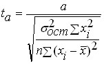 and
and 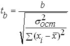
where: ![]()
![]() ,
, ![]() are the values of the Student’s criterion for the coefficients
are the values of the Student’s criterion for the coefficients ![]() and
and ![]() respectively;
respectively;
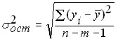 – residual variance of the regression equation
![]()
![]() – the number of points in the sample;
– the number of points in the sample;
![]()
![]() is the number of variables in the sample, for paired linear regression .
is the number of variables in the sample, for paired linear regression .![]()
The actual values of the Student’s criterion obtained are compared with the tabular values ![]()
![]() obtained from the Student’s distribution. If it turns out that
obtained from the Student’s distribution. If it turns out that ![]() , then the corresponding coefficient is statistically significant, otherwise it is not. The second option for checking the statistical significance of the coefficients is to determine the probability of occurrence of the Student’s
, then the corresponding coefficient is statistically significant, otherwise it is not. The second option for checking the statistical significance of the coefficients is to determine the probability of occurrence of the Student’s ![]() criterion and compare with the significance
criterion and compare with the significance ![]() level .
level .
For variables whose coefficients were not statistically significant, there is a high probability that their influence on the dependent variable in the general population is completely absent. For this reason, either it is necessary to increase the number of points in the sample, then perhaps the coefficient will become statistically significant and at the same time its value will be clarified, or as independent variables to find other, more closely related to the dependent variable. The accuracy of forecasting will increase in both cases.
As a rapid method for assessing the significance of the coefficients of the regression equation, the following rule can be used – if the Student’s criterion is greater than 3, then such a coefficient, as a rule, turns out to be statistically significant. In general, it is believed that in order to obtain statistically significant regression equations, it is necessary that the condition ![]()
![]() .
.
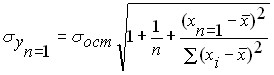
The standard prediction error for the obtained regression equation of an unknown value ![]()
![]() with a known one
with a known one ![]() is estimated by the formula:
is estimated by the formula:
Thus, a forecast with a confidence probability of 68% can be presented in the form of:
![]()
![]() .
.
If a different confidence probability ![]()
![]() is required, then for the significance
is required, then for the significance ![]() level it is necessary to find the Student’s
level it is necessary to find the Student’s ![]() criterion and the confidence interval for the prediction with the reliability
criterion and the confidence interval for the prediction with the reliability ![]() level will be
level will be ![]() .
.
Predicting multidimensional and nonlinear dependencies
If the predicted value depends on several independent variables, then in this case there is a multivariate regression of the form:
![]()
![]()
where: ![]()
![]() are regression coefficients that describe the effect of variables
are regression coefficients that describe the effect of variables ![]() on the predicted value.
on the predicted value.
The method of determining regression coefficients does not differ from paired linear regression, especially when using a spreadsheet, since the same function is used for both paired and multidimensional linear regression. In this case, it is desirable that there are no relationships between the independent variables, i.e. a change in one variable does not affect the values of other variables. But this requirement is not mandatory, it is important that there are no functional linear dependencies between the variables. The procedures described above for checking the statistical significance of the resulting regression equation and its individual coefficients, the estimation of the prediction accuracy remains the same as for the case of paired linear regression. At the same time, the use of multidimensional regressions instead of a pair usually allows, with the proper selection of variables, to significantly improve the accuracy of describing the behavior of the dependent variable, and hence the accuracy of forecasting.
In addition, the equations of multivariate linear regression make it possible to describe the nonlinear dependence of the predicted value on the independent variables. The procedure for reducing a nonlinear equation to a linear form is called linearization. In particular, if this dependence is described by a polynomial of degree other than 1, then, having replaced variables with degrees other than one with new variables in the first degree, we obtain a multidimensional linear regression problem instead of a nonlinear one. So, for example, if the influence of an independent variable is described by a parabola of the form
![]()
![]()
then the replacement ![]()
![]() allows you to convert the nonlinear problem to a multidimensional linear view
allows you to convert the nonlinear problem to a multidimensional linear view
![]()
![]()
Just as easily, nonlinear problems can be transformed in which nonlinearity arises due to the fact that the predicted value depends on the product of independent variables. To account for this influence, you must enter a new variable equal to this product.
In cases where nonlinearity is described by more complex dependencies, linearization is possible by transforming coordinates. To do this, values ![]()
![]() are calculated and graphs of the dependence of the source points in various combinations of transformed variables are constructed. That combination of transformed coordinates or transformed and untranslated coordinates in which the dependence is closest to the straight line suggests the replacement of variables that will lead to the transformation of a nonlinear dependence to a linear view. For example, a nonlinear dependence of the form
are calculated and graphs of the dependence of the source points in various combinations of transformed variables are constructed. That combination of transformed coordinates or transformed and untranslated coordinates in which the dependence is closest to the straight line suggests the replacement of variables that will lead to the transformation of a nonlinear dependence to a linear view. For example, a nonlinear dependence of the form
![]()
![]()
turns into a linear view
![]()
![]()
where: ![]()
![]() ,
, ![]() and .
and .![]()
The resulting regression coefficients for the transformed equation remain unbiased and efficient, but it is impossible to verify the statistical significance of the equation and the coefficients.
Testing the validity of the least squares method
The application of the method of least squares ensures the efficiency and non-bias of estimates of the coefficients of the regression equation under the following conditions (Gaus-Markov conditions):
1. ![]()
![]()
2. ![]()
![]()
3. Values ![]()
![]() are independent of each other
are independent of each other
4. Values ![]()
![]() do not depend on explanatory variables
do not depend on explanatory variables
The simplest way to verify that these conditions are met is by plotting residue graphs depending on , then on ![]()
![]() the independent (independent) variables. If the points on these graphs are located in a corridor symmetrically arranged on the abscissa axis and there are no patterns
the independent (independent) variables. If the points on these graphs are located in a corridor symmetrically arranged on the abscissa axis and there are no patterns ![]() in the location of the points, then the Gaus-Markov conditions are met and there are no opportunities to improve the accuracy of the regression equation. If this is not the case, then it is possible to significantly increase the accuracy of the equation and for this it is necessary to refer to the specialized literature.
in the location of the points, then the Gaus-Markov conditions are met and there are no opportunities to improve the accuracy of the regression equation. If this is not the case, then it is possible to significantly increase the accuracy of the equation and for this it is necessary to refer to the specialized literature.