To use the regression equation to predict, you have to calculate the coefficients and ![]()
![]() regression equations
regression equations![]() . And there is another problem that affects the accuracy of the prediction. It is that there are usually no all possible values of the variables X and Y, that is, the general set of the joint distribution in the forecasting problems is not known, only the sample from this general population is known. As a result, when forecasting is not a random component, in addition to the random component Another source of errors arises – errors caused by the incomplete correspondence of the sample of the general population and the errors generated by this in determining the coefficients of the regression equation.
. And there is another problem that affects the accuracy of the prediction. It is that there are usually no all possible values of the variables X and Y, that is, the general set of the joint distribution in the forecasting problems is not known, only the sample from this general population is known. As a result, when forecasting is not a random component, in addition to the random component Another source of errors arises – errors caused by the incomplete correspondence of the sample of the general population and the errors generated by this in determining the coefficients of the regression equation.
In other words, due to the fact that the general population is not known, the exact values of the coefficients and ![]()
![]() regression equations
regression equations ![]() cannot be determined. Using a sample from this unknown general population, one can only obtain estimates
cannot be determined. Using a sample from this unknown general population, one can only obtain estimates ![]() of both
of both ![]() the true coefficients
the true coefficients ![]() and
and![]() .
.
In order for forecasting errors as a result of such substitution to be minimal, the assessment must be carried out by a method that guarantees the non-bias and effectiveness of the values obtained. The method provides unbiased estimates if, with its repeated repetition with new samples from the same general population, the condition ![]()
![]() is met and
is met and ![]() . The method provides effective estimates if, with its repeated repetition with new samples from the same general population, a minimum variance of coefficients a and b is ensured, i.e. the conditions
. The method provides effective estimates if, with its repeated repetition with new samples from the same general population, a minimum variance of coefficients a and b is ensured, i.e. the conditions ![]() and
and ![]() .
.
In probability theory, the theorem has been proved according to which the efficiency and non-bias of the estimates of the coefficients of the linear regression equation according to the sample data is ensured by applying the method of least squares.
The essence of the method of least squares is as follows. For each of ![]()
![]() the sampling points, an equation of the form
the sampling points, an equation of the form ![]() is written . Then there is an error
is written . Then there is an error ![]() between the calculated and actual values
between the calculated and actual values![]() . Solving the optimization problem of finding such values
. Solving the optimization problem of finding such values ![]() and
and ![]() which provide a minimum sum of squared errors for all n points, i.e. solving the search
which provide a minimum sum of squared errors for all n points, i.e. solving the search ![]() problem , gives unbiased and effective estimates of the coefficients and
problem , gives unbiased and effective estimates of the coefficients and ![]() . For the case of paired linear regression
. For the case of paired linear regression![]() , this solution is of the form:
, this solution is of the form:
![]()
It should be noted that the unbiased and effective estimates of the true values of the regression coefficients for the general population obtained in this way from the sample do not guarantee against error in a single application. The guarantee is that, as a result of repeated repetition of this operation with other samples from the same general population, a smaller amount of errors is guaranteed compared to any other method and the spread of these errors will be minimal.
The obtained coefficients of the regression equation determine the position of the regression line, it is the main axis of the cloud formed by the points of the initial sample. Both coefficients have a very definite meaning. The coefficient ![]()
![]() shows the value
shows the value ![]() at
at ![]() , but in many cases
, but in many cases ![]() does not make sense, and often
does not make sense, and often ![]() also does not make sense, so the above interpretation of the coefficient
also does not make sense, so the above interpretation of the coefficient ![]() should be used carefully. A more universal interpretation of the meaning
should be used carefully. A more universal interpretation of the meaning ![]() is as follows. If
is as follows. If ![]() , then the relative change in the independent variable (the change in percentage) is always less than the relative change in the dependent variable.
, then the relative change in the independent variable (the change in percentage) is always less than the relative change in the dependent variable.
The coefficient ![]()
![]() shows how much the dependent variable will change when the independent variable changes by one unit. The coefficient
shows how much the dependent variable will change when the independent variable changes by one unit. The coefficient ![]() is often called the regression coefficient, emphasizing that it is more important than
is often called the regression coefficient, emphasizing that it is more important than ![]() . In particular, if you take their deviations from their average values instead of the values of the dependent and independent variables, then the regression equation is transformed to the form
. In particular, if you take their deviations from their average values instead of the values of the dependent and independent variables, then the regression equation is transformed to the form ![]() . In other words, in the transformed coordinate system, any regression line passes through the origin (Figure 13) and there is no coefficient
. In other words, in the transformed coordinate system, any regression line passes through the origin (Figure 13) and there is no coefficient ![]() .
.
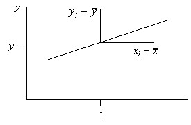
Fig. 13. The position of the regression dependency in the transformed coordinate system.
The parameters of the regression equation tell us how the dependent and independent variable are related, but say nothing about the degree of closeness of the connection, i.e. show the position of the main axis of the data cloud, but do not say anything about the degree of closeness of the connection (how narrow or wide the cloud is).
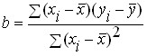
The degree of closeness of the connection can be judged by the linear correlation ![]()
![]() coefficient:
coefficient:

The correlation coefficient varies from -1 to +1. The closer it is in absolute value to one, the stronger the dependence (the more the data cloud is pressed against its main axis). If ![]()
![]() the slope of the regression line is negative, the closer it is to 0, the weaker the bond, with
the slope of the regression line is negative, the closer it is to 0, the weaker the bond, with ![]() a linear relationship between the variables there is no relationship, and when
a linear relationship between the variables there is no relationship, and when ![]() the relationship of variables is functional. The effect of the correlation coefficient on the shape and position of the data cloud is illustrated in Figure 14.
the relationship of variables is functional. The effect of the correlation coefficient on the shape and position of the data cloud is illustrated in Figure 14.
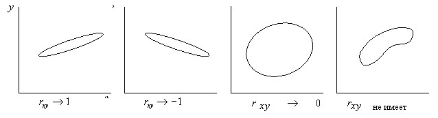
Fig. 14. The influence of the shape and position of the data cloud on the paired linear correlation coefficient.
The correlation coefficient allows you to get an estimate of the accuracy of the regression equation – the coefficient of ![]()
![]() determination. For paired linear regression, it is equal to the square of the correlation coefficient, for multivariate or nonlinear regression
determination. For paired linear regression, it is equal to the square of the correlation coefficient, for multivariate or nonlinear regression ![]() it is more difficult to determine. The coefficient of determination shows how many percent of the variance of the dependent variable is explained by the regression equation, and
it is more difficult to determine. The coefficient of determination shows how many percent of the variance of the dependent variable is explained by the regression equation, and ![]() – how many percent of the variance remained unexplained (depends on the random term
– how many percent of the variance remained unexplained (depends on the random term ![]() we do not control) ).
we do not control) ).