The easiest way to characterize the accuracy of the forecast is to indicate the extent of fluctuations in the values of a random variable in the sample. The range of oscillations is the difference between the maximum and minimum values, the larger it is, the lower the accuracy of the forecast. But this characteristic has a significant drawback – in the presence of emissions (abnormally large and abnormally small values), the scope of oscillations underestimates the accuracy estimate, since it reacts only to them.
A more objective characteristic of the randomness of a random variable would be either the sum of the random variable’s deviations from its mean or, better yet, the average of that deviation. But because the random variable’s deviations from the mean can be both positive and negative, the sum tends to tend to zero. To eliminate this disadvantage, you must use either the absolute values of these deviations or squares. Deviations. Absolute values represent less opportunities for theoretical constructions, so historically dispersion is used as the main measure of the oscillation of a random variable. Variance is the average square of a random variable’s deviation from its mean. For the general population, the variance is determined by the formula:
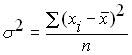
where: ![]()
![]() is the i-th value from the general population of a random variable;
is the i-th value from the general population of a random variable;
![]()
![]() – its average value;
– its average value;
![]()
![]() is the number of random variable values in the population.
is the number of random variable values in the population.
Another version of the formula for calculating variance, convenient for manual counting or in the case when new values of a random variable appear, is:
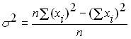 .
.
In the case when the general population is not known, and only a sample from it is known, then the estimation of the variance of the general population from the sample data should be made according to slightly modified formulas:
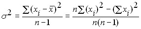 .
.
Variance is a universal indicator of the degree of oscillability of a random variable, and hence the accuracy of the forecast, but it has a significant drawback – this value essentially has no units of measurement (profit is measured in rubles, profit variance is rubles squared). Therefore, along with the variance, to characterize the oscillation of the initial data, a value derived from the variance is used – the standard deviation (the second name is the standard deviation) ![]()
![]() equal to the square root of the variance, i.e.:
equal to the square root of the variance, i.e.:
![]()
![]() .
.
Unlike variance, the standard deviation has the same dimension as the random variable it characterizes.
To fully characterize the accuracy of the resulting prediction, the variance or standard deviation alone is not enough, it is also necessary to specify the type of distribution of the random variable.
If you take a histogram of a random variable and begin to increase the number of intervals at which it is built (reduce their value), then the histogram will begin to decrease in height and become smoother (Fig. 7). With an infinitely large number of random variable values and an infinitesimal value of intervals, the histogram will turn into a smooth curve. The curve obtained in this way is called the distribution density curve or the second name is the distribution density function.
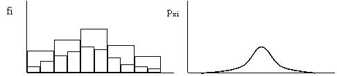
Fig. 7. Scheme for obtaining a distribution density curve.
The height of the density curve of the distribution shows the probability of the occurrence of a given value of a random variable. The area under the density curve of the distribution is assumed to be equal to one. This is the probability of any random variable appearing in the range from ![]()
![]() to
to ![]() . Then the ratio of the area of the figure of the limited density curve of the distribution and the two vertical segments passing through
. Then the ratio of the area of the figure of the limited density curve of the distribution and the two vertical segments passing through ![]() and
and ![]() to the area of the whole figure under the density curve of the distribution is equal to the probability of the appearance of the next value of the random variable in the range from
to the area of the whole figure under the density curve of the distribution is equal to the probability of the appearance of the next value of the random variable in the range from ![]() to
to ![]() (Fig. 8, a).
(Fig. 8, a).
In the limit ![]()
![]() can be equal
can be equal ![]() to , then the area of the left side of the figure will be equal to the probability of the appearance of the next value of a random variable less than or equal
to , then the area of the left side of the figure will be equal to the probability of the appearance of the next value of a random variable less than or equal ![]() (Fig. 8, b). In the case when
(Fig. 8, b). In the case when ![]() =
= ![]() , then the right part of the figure will be equal to the probability of the appearance of the next value of a random variable greater or equal
, then the right part of the figure will be equal to the probability of the appearance of the next value of a random variable greater or equal ![]() (Fig. 8, c).
(Fig. 8, c).
In addition to the distribution density function, a function can be used to characterize the type of distribution that shows the probability of occurrence of another random variable value less than or equal to a given value. This is a cumulative (accumulated) distribution function. The points on the distribution curve are the values of the area under the distribution density curve in the range from ![]()
![]() to
to ![]() , in other words they are equal to the integral
, in other words they are equal to the integral
![]()
![]()
where: ![]()
![]() is the distribution density function.
is the distribution density function.
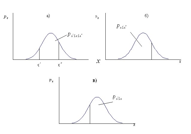
Fig. 8. Use the density curve to determine the probability of occurrence of the next value of a random variable in a given range.
According to the graph of the cumulative distribution curve, in addition to the probability of the appearance of the random variable value within the given limits, it is possible to determine its expected value (such ![]()
![]() as , for which the distribution function is 0.5), the expected loss (
as , for which the distribution function is 0.5), the expected loss (![]() ) and the expected income (
) and the expected income (![]() ). The expected loss is the distance from the axis of ordinate to the center of gravity of the figure formed by the distribution function and the axes of coordinates. The expected income is the distance from the axis of ordinate to the center of gravity of the figure formed by the axis of gravity ordinate, a distribution function and a horizontal line passing through 1 on the axis of the ordinate (Fig. 9).
). The expected loss is the distance from the axis of ordinate to the center of gravity of the figure formed by the distribution function and the axes of coordinates. The expected income is the distance from the axis of ordinate to the center of gravity of the figure formed by the axis of gravity ordinate, a distribution function and a horizontal line passing through 1 on the axis of the ordinate (Fig. 9).

Fig. 9. Use the distribution function to find the expected gain and loss.
Mathematically, the expected loss is

a expected income

There are many types of random variable distribution, but the most common in practice is the normal distribution. Its greatest prevalence is mathematically proven. According to one of the variants of the ultimate theorem of probability theory, if the random variable under study depends on many other random variables and among these influencing quantities there are no prevailing forces of influence, then the studied random variable will have a distribution close to normal, regardless of what distributions the influencing quantities have.
The normal distribution takes the form of a bell-shaped symmetric curve, the highest point of which corresponds ![]()
![]() to , and the height and width are determined by
to , and the height and width are determined by ![]() the value . The density function of the normal distribution is described by the dependence of the form:
the value . The density function of the normal distribution is described by the dependence of the form:
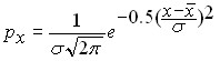
Figure 10 shows the density curves of the normal distribution of three random variables illustrating the effect of the parameters of the random variable on the density curve of the normal distribution. As follows from these graphs, the position of the curve on the numerical axis is determined by the average value of the random variable – the median of the density curve of the normal distribution corresponds, and the shape of the curve – its height and width – are determined by the standard deviation ![]()
![]() .
.
Fig. 10. The influence of random variable parameters on the position and shape of the density curve of the normal distribution.
Depending on the specific values ![]()
![]() ,
, ![]() there are countless variations of the density curve of the distribution. However, due to the algebraic transformation of a random variable, all this manifold can be reduced to one single variant.
there are countless variations of the density curve of the distribution. However, due to the algebraic transformation of a random variable, all this manifold can be reduced to one single variant.
If we subtract its average value from the values of a random variable, i.e. replace the coordinate with ![]()
![]() , then all the density curves of the distribution are arranged symmetrically to
, then all the density curves of the distribution are arranged symmetrically to ![]() the ordinate axis (Fig. 11a). The differences between them are preserved only in height and width. The height of each of them is equal
the ordinate axis (Fig. 11a). The differences between them are preserved only in height and width. The height of each of them is equal ![]() and when
and when ![]() it becomes equal
it becomes equal ![]() to , i.e. the random variable turns into an ordinary deterministic. Another transformation consisting
to , i.e. the random variable turns into an ordinary deterministic. Another transformation consisting ![]() in division the standard deviation causes the density curves of the normal distributions of any random variable to be converted to a single curve, the probability density function of the standardized normal distribution.
in division the standard deviation causes the density curves of the normal distributions of any random variable to be converted to a single curve, the probability density function of the standardized normal distribution.
On the horizontal axis in this case, it is not the values of a random variable that are deposited, but their dimensionless analogues, measured in standard deviations.
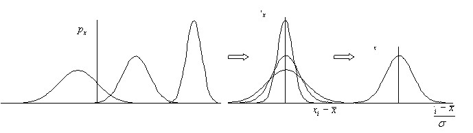
Fig. 11. Convert the normal distribution to a standardized form.
The density curve of the standardized normal distribution has been studied in detail. Its values, as well as the values of the cumulative function, are given in almost all textbooks on probability theory and statistics. This makes it easy to calculate the probability of occurrence of an event for any random variable having a normal distribution. So, for example, to determine the probability of occurrence of the next value of a random variable equal, it is necessary to find ![]()
![]() , further on the table of the probability density of the standard normal distribution
, further on the table of the probability density of the standard normal distribution ![]() to find this probability. If you want to find the probability that the next value of
to find this probability. If you want to find the probability that the next value of ![]() the random variable will not exceed
the random variable will not exceed ![]() , then again it is necessary to first make the transition from
, then again it is necessary to first make the transition from ![]() to
to ![]() and then look for this probability in the table of the appearance of the next value of a random variable in the range from
and then look for this probability in the table of the appearance of the next value of a random variable in the range from ![]() to . The only difficulty encountered in this case is that different sources give different variants of the range for which the probability of occurrence of a random quantity in a given range is calculated. This range can be in the classical form from
to . The only difficulty encountered in this case is that different sources give different variants of the range for which the probability of occurrence of a random quantity in a given range is calculated. This range can be in the classical form from![]()
![]() ; from 0 to
; from 0 to ![]()
![]() , From
, From ![]() to
to ![]() . In the event that the probability calculations are carried out in a spreadsheet, then the problem is greatly simplified, because it has a special function that allows, without using the z transformation, to calculate the probability of the appearance of a given value of a random variable or that it will not exceed a given value. All other options are easily found according to the scheme of Fig. 6.
. In the event that the probability calculations are carried out in a spreadsheet, then the problem is greatly simplified, because it has a special function that allows, without using the z transformation, to calculate the probability of the appearance of a given value of a random variable or that it will not exceed a given value. All other options are easily found according to the scheme of Fig. 6.
The probability that the next value of a random variable will be no less than ![]()
![]() is according to the formula:
is according to the formula:
![]()
![]() ,
,
the probability that the next value of a random variable will be in the range from ![]()
![]() to
to ![]() – according to the formula:
– according to the formula:
![]()
![]() ,
,
outside this range:
![]()
![]()
For rapid estimates of the probability of occurrence of an event, it is useful to know some basic relationships for the normal distribution:
the probability of the next random variable falling into the interval
![]()
![]() is ≈ 68.3%, i.e. the odds are approximately 2 to 1
is ≈ 68.3%, i.e. the odds are approximately 2 to 1
![]()
![]() is ≈ 95.5%, i.e. the odds are approximately 20 to 1
is ≈ 95.5%, i.e. the odds are approximately 20 to 1
![]()
![]() is 99.7%, i.e. the odds are approximately 300 to 1.
is 99.7%, i.e. the odds are approximately 300 to 1.
Or another option, more convenient for practice:
there is a 10% probability that the next value will be out of bounds ![]()
![]() (1 chance out of 10);
(1 chance out of 10);
5% probability of going beyond the limits ![]()
![]() (1 chance out of 20);
(1 chance out of 20);
1% probability of going beyond the limits ![]()
![]() (1 chance out of 100).
(1 chance out of 100).
When working with samples, the question always arises as to whether the distribution chosen for calculations is justified and what are the errors with the wrong type of distribution. The Russian mathematician Chebyshev proved the theorem that in the case of any distribution, the probability of the next value going beyond the limits ![]()
![]() does not exceed 10%. In other words, any errors in the choice of the distribution threaten us with errors not exceeding 10%, while attempts to estimate the probability “by eye” are obviously fraught with much more significant misses.
does not exceed 10%. In other words, any errors in the choice of the distribution threaten us with errors not exceeding 10%, while attempts to estimate the probability “by eye” are obviously fraught with much more significant misses.
In conclusion, we note that the problem of predicting a random variable from a sample of its previous values or from values characteristic of objects of the same class is reduced to:
to find the median, mean or mode of the serving as the forecast value;
specifying the limits and probability of the forecast falling within these limits as a characteristic of the accuracy of the forecast.
As an alternative way to characterize the accuracy of the forecast, you can specify the probability of obtaining and the expected value of the negative value of the predicted value and the probability and expected value of the positive value.