It should be considered generally recognized that over time in an enterprise that maintains a fixed number of employees and a constant amount of fixed assets, output increases. This means that in addition to the usual production factors associated with the cost of resources, there is a factor that is usually called scientific and technological progress (STP). This factor can be considered as a synthetic characteristic that reflects the combined impact on economic growth of many significant phenomena, among which the following should be noted:
(a) the improvement over time of the quality of the labour force, as a consequence of the upgrading of the skills of workers and their mastery of the use of improved technology;
b) improving the quality of machinery and equipment leads to the fact that a certain amount of capital investment (in constant prices) allows you to purchase a more efficient machine after a while;
c) improvement of many aspects of the organization of production, including the improvement of supply and sales, banking operations and other mutual settlements, the development of the information base, the formation of various kinds of associations, the development of international specialization and trade, etc.
In this regard, the term “scientific and technological progress” can be interpreted as a set of all phenomena that, with fixed quantities of production factors spent, make it possible to increase the output of high-quality, competitive products. The very vague nature of this definition leads to the fact that the study of the impact of NTP is carried out only as an analysis of the additional increase in production, which cannot be explained by a purely quantitative increase in production factors. The main approach to accounting for NTP is that time (t) as an independent production factor is introduced into the set of characteristics of output or costs, and the transformation in time of either the production function or the technological set is considered.
Let us dwell on the ways of accounting for NTP by transforming the production function (PF), and we will take the two-factor PF as a basis.
y= f(K,L),
where capital (K) and labor (L) are the factors of production. Modified PF in the general case has the form:
y= f(K,L,t),
and the following condition is met:

which reflects the fact of growth of production over time with fixed costs of labor and capital. A geometric illustration of such a process is given in Figure 6.13, which shows that the isoquant corresponding to the output in the volume Q shifts over time (t2>t1) down and to the left.
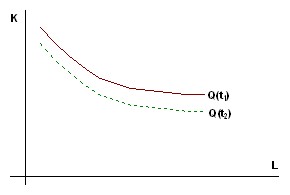
Rice. 6.13. Growth of production over time with fixed costs of labor and capital
When developing specific modified PFs, it is usually sought to reflect the nature of the NTP in the observed situation. In this case, four cases are distinguished:
(a) A significant improvement over time in the quality of the workforce results with fewer employees; this type of NTP is often called labor-saving. Modified PF has the form:
y= f(K, l(t)L),
where the monotonic function l(t) characterizes the growth of labor productivity;
b) the preferential improvement in the quality of machinery and equipment increases the return on capital, there is a capital-saving NTP and the corresponding PF as follows:
y= f(k(t)K,L),
where the increasing function k(t) reflects the change in return on capital;
c) if there is a significant influence of both mentioned phenomena, then the PF is used in the form of:
y= f(k(t)K,l(t)L);
d) if it is not possible to identify the influence of NTP on production factors, then the PF is applied in the form of:
y= a(t) f(K,L),
where a(t) is an increasing function that expresses the growth of production at constant values of the inputs of the factors.
To study the properties and features of NTP, some correlations between the results of production and the costs of factors are used. These include:
(a) Average labour productivity

b) average return on capital

c) the coefficient of the employee’s capital-labor ratio

d) equality between the level of remuneration and marginal (marginal) labour productivity

e) equality between the maximum return on capital and the rate of bank interest

A NTP is said to be neutral if it does not change certain relationships between the values given over time.
Consider three cases below.
1) Progress is called Hicks-neutral if the ratio between the capital-to-weight ratio (x) and the marginal rate of substitution of factors (w/r) remains unchanged over time. In particular, if w/r = const, then the replacement of labor with capital and vice versa will not bring any benefit and the capital-labor ratio ![]()
![]() will also remain constant. It can be shown that in this case the modified PF has the form:
will also remain constant. It can be shown that in this case the modified PF has the form:
y= a(t)f(K,L) ,
and Hicks neutrality is equivalent to the effect of NTP directly on output discussed above. In the situation under consideration, the isoquant shifts to the left downwards over time by transforming the similarity, i.e. remains in exactly the same shape as in the original position;
2) progress is called neutral according to Harrod, if during the period in question the rate of bank interest (r) depends only on the return on capital (k), i.e. it is not affected by the NTP. This means that the marginal return on capital is set at the level of the interest rate and further increase in capital is impractical. It can be shown that this type of NTP corresponds to the production function
y= f(K,l(t)L),
i.e. technological progress is labor-saving;
(3) Progress is Solow-neutral if equality between pay (w) and marginal labour productivity remains unchanged and further increases in labour input are not profitable. It can be shown that in this case the PF has the form:
y= f(k(t)K,L),
i.e. NTP turns out to be fund-saving. Let’s give a graphical representation of three types of NTP on the example of a linear production function:
y= bK + cL (b>0, c>0).
In the case of Hicks neutrality, we have a modified PF:
y= a(t) (bK+cL),
where a(t) is an increasing function t. This means that over time, the isoquant Q (the segment of the line AB) shifts to the origin by a parallel transfer (Figure 6.14) to the position A1B1.
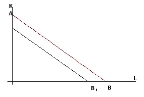
Rice. 6.14. Isocquant shift at neutral Hicks NTP
In the case of Harrod neutrality, the modified PF is:
y= bK + cl(t)L,
where l(t) is an increasing function.
Obviously, over time, point A remains in place and the isoquant is shifted to the origin by rotating to position AB1 (Figure 6.15).
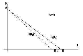
Rice. 6.15. Isocquant shift in labor-saving NTP
For progress neutral on Solow, the corresponding modified PF:
y= bk(t)K + cL,
where k(t) is an increasing function. The isoquant shifts to the origin, but point B does not shift, and the rotation to position A1B occurs (Figure 6.16).
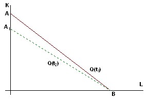
Rice. 6.16. Isovant shift in capital-saving NTP
When constructing production models taking into account NTP, the following approaches are mainly used:
(a) An idea of exogenous (or autonomous) technological progress, which also exists when the underlying factors of production do not change. A special case of such a NTP is the neutral Hicks progress, which is usually accounted for by an exponential multiplier, for example:
![]()
![]()
It ![]()
![]() is not difficult to see that time here acts as an independent factor in the growth of production, but it seems that the NTP occurs on its own, without requiring additional labor and capital investment;
is not difficult to see that time here acts as an independent factor in the growth of production, but it seems that the NTP occurs on its own, without requiring additional labor and capital investment;
b) the idea of technical progress embodied in capital, connects the growth of the influence of NTP with the growth of capital investments. To formalize this approach, the model of progress of the neutral according to Solow is taken as a basis:
y= f(k(t)K,L),
which is written as
![]()
![]()
where ![]()
![]() are the fixed assets at the beginning of the period,
are the fixed assets at the beginning of the period,
![]()
![]() – accumulation of capital during the period equal to the amount of investment.
– accumulation of capital during the period equal to the amount of investment.
Obviously, if the investment is not made, then ![]()
![]() , and the increase in output due to the NTP does not occur;
, and the increase in output due to the NTP does not occur;
c) the approaches to modeling NTP discussed above have a common feature: progress acts as an exogenously specified value that affects labor productivity or capital return and thereby affects economic growth.
In the long term, however, STP is both the result of development and, to a large extent, its cause. Since it is economic development that allows rich societies to finance the creation of new models of technology, and then reap the benefits of the scientific and technological revolution. Therefore, the approach to NTP as an endogenous phenomenon caused by (induced) economic growth is quite legitimate.
There are two main directions of modeling of NTP.
1) The model of induced progress is based on the formula:
y= f(k(t)K,l(t)L),
it is assumed that the company can distribute investments intended for NTP between its various directions. For example, between the growth of capital return (k(t)) (improving the quality of machines) and the growth of labor productivity (l(t)) (improving the skills of employees) and choosing the best (optimal) direction of technical development with a given amount of allocated capital investments.
2) The model of the learning process in the course of production, proposed by C. Arrow, is based on the observed fact of the mutual influence of the growth of labor productivity and the number of new inventions. In the course of production, workers gain experience, and the time to manufacture the product decreases, i.e. labor productivity and the labor contribution itself depend on the volume of production. ![]()
![]()
In turn, the growth of the labor factor according to the production function y = f(K,L) leads to an increase in production. In the simplest version of the model, the following formulas are used:
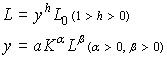
(Cobb-Douglas production function).
Hence we have the ratio:
![]()
![]()
which, given the functions K(t) and L0(t), shows faster growth y due to the above-mentioned mutual influence of NTP and economic development.
Let’s say, for example: ![]()
![]()
Then growth without taking into account mutual influence is described by the equation:
![]()
![]()
and growth, taking into account the mutual influence of the equation:
![]()
![]()
or
![]()
![]() ,
,
i.e. it turns out to be much faster.
For a linear model:
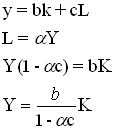 ,
,
i.e. the return on capital increases.