Modeling of costs and profits of the enterprise

The basis for the construction of models of behavior of the producer (an individual enterprise or firm, an association or an industry) is the idea that the producer seeks to achieve such a state in which he would be provided with the greatest profit under the prevailing market conditions, i.e. primarily under the existing price system.

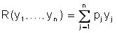
The simplest model of the optimal behavior of the manufacturer in conditions of perfect competition is as follows: let the enterprise (firm) produce one product in the amount of y physical units. If p is the exogenously set price of this product and the firm sells its output in full, then it receives gross income (revenue) in the amount of:

R(y)=py.

In the process of creating this quantity of product, the firm incurs production costs in the amount of C(y). At the same time, it is natural to assume that C′(y)>0, i.e. costs increase with increasing production volume. It is also commonly believed that C′′(y)>0. This means that the additional (marginal) cost of producing each additional unit of output increases as the volume of production increases. This assumption is due to the fact that with rationally organized production, with small volumes, the best machines and highly qualified workers can be used, which will no longer be at the disposal of the firm when the volume of production increases. In Fig. Figure 6.10 shows typical graphs of the functions R(y) and C(y). Production costs consist of the following components:

1) material costs cm, which include costs for raw materials, materials, semi-finished products, etc.

The difference between gross income and material costs is called value added (value added).

VA = Z = R – Cm;

2) cl labor costs;

3) expenses related to the use, repair of machinery and equipment, depreciation, the so-called payment for “capital services” Ck;

(4) Cr’s additional costs related to the expansion of production, the construction of new buildings, access roads, communication lines, etc.

Total production costs:

C = Cm + Cl + Ck + Cr

As noted above

C = C(y),

however, this dependence on the volume of output (y) for different types of costs is different. Namely, there are:

a) fixed costs C0, which are practically independent of y, including payment of administrative staff, rental and maintenance of buildings and premises, depreciation, interest on credit, communication services, etc.:

b) proportional to the volume of output (linear) costs C1, this includes material costs Cm, remuneration of production personnel (part Cl), maintenance costs of operating equipment and machines (part Ck), etc.

C1 = ay,

where a is a generalized indicator of the costs of these types per product;

c) “super-proportional” (non-linear) costs of C2, which include the acquisition of new machines and technologies, i.e. costs of type Cr), overtime pay, etc. For a mathematical description of this type of cost, a power dependence is usually used:

C2 = byh  (h > 1).

Therefore, you can use a model to represent total costs.

C(y) = C0 + C1 + C2 = C0 + ay + byh.  (2.1).

(Note that the conditions C′(y)>0, C′′′(y)>0 for this function are satisfied).

Consider the possible options for the behavior of an enterprise (firm) for two cases:

1) The enterprise has a sufficiently large reserve of production capacity and does not seek to expand production, so it can be assumed that C2 = 0 and total costs are a linear function of the output volume:

C(y) = C0 + ay

Profit will be:

P(y) = R – C = py – (C0 + ay).

Obviously, with small volumes of issue 0 ≤ y ≤ yw , the company incurs losses, because P < 0.

Here yw is the break-even point (profitability threshold) determined by the ratio P(yw) = 0.

If y > yw, the firm makes a profit and the final decision on the volume of output depends on the state of the market for the products (Figure 6.10).

In this case, there are two break-even points , and the firm will receive a positive profit if the volume of output of Y , satisfies the condition .

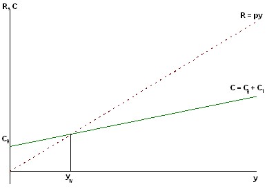
Rice. 6.10. Lines of revenue and expenses of the enterprise

At this point, the greatest value of profit is reached at the point , so there is an optimal solution to the problem of maximizing profits. At point A, corresponding to costs at optimal output, the tangent to the cost curve C parallels the straight line of income R.

It should be noted that the final decision of the firm also depends on the state of the market, but from the point of view of observing economic interests, it should recommend the optimizing value of output (Fig. 6.11).

In general, when C(y) is a nonlinear increasing and downward convex function (because.C′(y)>0 and C′′′(y)>0) of the output volume, the situation is completely similar to that discussed in paragraph 2. By definition, profit is considered to be the value of P(y) = R(y) – C(y).

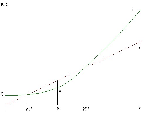
Fig. 6.11. Optimal volume of output

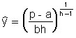
The break-even points , are determined from the condition of equality of profit to zero, and its maximum value is reached at the point , which satisfies the equation:

P′() = 0 or R′() – C′() = 0.

Thus, the optimal volume of production is characterized by the fact that in this state the marginal gross income (R′(y)) is exactly equal to the marginal costs of C′(y).

Indeed, if y < , then R′(y) > C′ (y), and then output should be increased, since the expected additional income will exceed the expected additional costs. If y > , then R′(y) < C′(y), and any increase in volume will reduce profits, so it is natural to recommend reducing output and coming to the state of y = (Fig. 6.12).

Rice. 6.12. Profit maximum point and break-even zone:

(*).

It is not difficult to see that as the price (p) increases, the optimal output  (as well as profit) increases, i.e., as the price (p) increases.

This is also true in the general case, because…

Example. The company produces agricultural machines in the  number of pieces, and the volume of production in principle can vary from 50 to 220 pieces per month. At the same time, of course, an increase in production volume will require an increase in costs, both proportional and super-proportional (nonlinear), since it will be necessary to purchase new equipment and expand production areas.

In a specific example, we will proceed from the fact that the total costs (cost) for the production of products in the quantity of products are expressed by the formula:

C(y) = 1000 + 20y + 0.1y2 (thousand rubles).

This means that fixed costs C0 = 1000 (i.e. rubles) are proportional costs C1 = 20y, i.e. the generalized indicator of these costs per product is a = 20 thousand rubles; and the nonlinear cost would be C2 = 0.1y2 (b = 0.1).

The above formula for costs is a special case of the general formula, where the indicator h = 2.

To find the optimal volume of production, we will use the formula of the maximum profit point (*), according to which we have:

.

It is obvious that the volume of production at which the maximum profit is achieved is very significantly determined by the market price of the product P.

In the table below, the results of calculating the optimal volumes at different price values from 40 to 60 thousand rubles per product are presented.

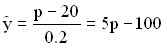
The first column of the table shows the possible output volumes of y, the second column contains data on the total costs of C(s), the third column shows the cost price per product:

.

The fourth column characterizes the values of the above marginal costs of the MS, which show how much it costs to produce one additional product in a given situation. It is easy to see that marginal costs increase as production increases, which is well consistent with the point made at the beginning of this paragraph. When considering the table, it should be noted that the optimal volumes are exactly at the intersection of the row (marginal costs – MS) and the column (price – P) with their equal values, which is quite accurately correlated with the rule of optimality established above.

The above analysis refers to an environment of perfect competition, when the producer cannot influence the price system by his actions, and therefore the price P for the product U acts in the manufacturer’s model as an exogenous quantity.

Table 6.1 Resource requirements by component

Data on output, costs and profits

In the case of imperfect competition, the producer can have a direct influence on the price. This is especially true for the monopoly producer of the commodity, which forms the price for reasons of reasonable profitability.

Consider a firm with a linear cost function that determines the price in such a way that the profit is a certain percentage (a share of 0 < γ < 1) of gross income, i.e.:

.

Hence we have:

.

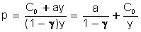Gross income:

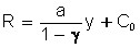
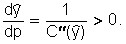
And production turns out to break even, starting with the smallest volumes of production (). It is easy to see that the price depends on the volume, i.e. p = p(y) and with an increase in the volume of production (y), the price of the commodity decreases, i.e. This situation is the case for the monopolist and in the general case.

The requirement to maximize profits for the monopolist is as follows:

Assuming still that , we have an equation for finding the optimal output ()

It is useful to note that the optimal output of a monopolist () is generally not superior to the optimal output of a competing producer in the formula (*).

A more realistic (but also simple) model of the company is used to take into account resource constraints, which play a very large role in the economic activities of manufacturers. The model identifies one of the most scarce resources (labor, fixed assets, rare material, energy, etc.) and assumes that the firm can use it no more than in the amount of Q. The firm can produce n different products. Let y1,…, yj,…, yn be the desired production volumes of these products; p1,…, pj,…, pn are their prices. Let also q be the unit price of the scarce resource,  and then the firm’s gross income is

  ,

and the profit will be

  .

It is easy to see that with fixed q and Q, the problem of maximizing profits is transformed into the task of maximizing gross income.

Suppose further that the resource overhead function for each product Cj(yj) has the same properties that were expressed above for the C(y) function. Thus, and .

In its final form, the model of optimal behavior of a firm with one limited resource is as follows:

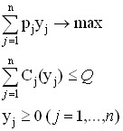
It is not difficult to see that, in a fairly general case, the solution to this optimization problem is by investigating a system of equations:

  (**)

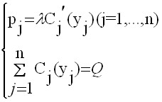where λ is the Lagrange multiplier.

Note that the ratio is essentially analogous to the above-mentioned coincidence at the optimal point of marginal income and marginal costs. In the case of quadratic cost functions from the system (**) we have:

(***)

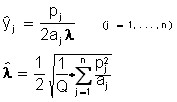Note that the optimal choice of the company depends on the totality of prices for products (p1,…,pn); moreover, this choice is a homogeneous function of the price system, i.e. with a simultaneous change in prices by the same number of times, the optimal outputs do not change. It is also easy to see that from (***) it follows that when the price of product j increases (with constant prices for other products), its output should be increased in order to maximize profits, i.e.:

,

and the production of the remaining goods will decrease, i.e., the production of the remaining goods will decrease.

.

These ratios collectively show that in a given model, all products are competing. From the formula (***) also follows the obvious relation:

,

i.e. with an increase in the volume of the resource (capital investment, labor, etc.), the optimal outputs increase.

In conclusion of the paragraph, we will give a number of simple examples that will help to better understand the rule of the optimal choice of a company on the principle of maximum profit:

1) let n = 2; p1 = p2 = 1; a1 = a2 = 1; Q = 0.5; q = 0.5.

Then from (***) we have:

2) let now all the conditions remain the same, but the price of the first product has doubled: p1 = 2.

Then the optimal profit plan of the company:

The expected maximum profit increases markedly:

3) note that in the previous example 2, the firm must change the volume of production, increasing the production of the first and reducing the production of the second product. Suppose, however, that the company does not pursue the maximum profit and does not change the established production, i.e. chooses the program y1 = 0.5;  y2 = 0.5.

It turns out that in this case the profit will be P = 1.25. This means that when prices rise in the market, a firm can get a significant increase in profits without changing the output plan.