Market demand is determined on the basis of decisions that are made by many individuals, based on their needs and disposable incomes. But in order to distribute funds between various needs, it is necessary to somehow compare them. As a basis for comparing different needs at the end of the nineteenth century, economists adopted utility. The term “utility” itself was introduced by the English philosopher I. Bentham (1748-1832). According to Bentham, maximizing utility is the guiding psychological principle of human behavior. The category of utility was adopted by economists and formed the basis of the theory of consumer behavior, which in turn is based on the hypothesis of the comparability of the usefulness of a wide variety of goods. It was believed that at given prices, consumers tend to allocate their funds for the purchase of various goods in such a way as to maximize the expected satisfaction or usefulness from their consumption. At the same time, they are guided by their personal tastes and ideas.
Economists in the second half of the nineteenth century put forward two approaches to comparing and measuring the utility of various goods – quantitative and ordinal.
Almost simultaneously, the English economist Stanley Jevons, the Austrian economist Carl Menger (1840-1921) and the Swiss economist Leon Walras proposed the quantitative theory of utility. At the heart of this theory was the hypothesis that it is possible to measure different goods. This theory was shared by A. Marshall.
However, this theory has met with serious criticism. The English economist Francis Edgeworth (1845-1926), Wilfredo Pareto, and the American economist Irving Fisher proposed an alternative quantitative ordinal theory of utility, which is now the most common.
Models of consumer behavior and demand are based on income distribution models and utility theory. Let’s first consider the models of income distribution.
The construction of personal consumption models is based on the principle of distribution of consumers into groups, for the formation of which both data on the social status of families and information on their incomes are used. In accordance with this approach, the entire set of consumers, i.e. the population of a country or region, is considered as a set of several groups of families, each of which is characterized by a certain level of income and approximately the same social status (employees, workers, peasants, etc.). At the same time, it is believed that each such group has some commonality in the choice and preference of certain consumer goods. When dividing consumers into groups at different income levels, different types of income distribution models are usually used.
To characterize the uniformity of the distribution of income in society, the so-called Lorentz curve is often used. It is built as follows: the entire set of consumers of a given country or region is divided into a certain number of groups, usually equal in number, but different in income. The share of national income received by each such group is then calculated, with the account kept starting with the group with the lowest income upwards.
Further in the diagram (Fig. 5.1.) the dots corresponding to the calculated percentages shall be plotted. Obviously, a straight line corresponds to a completely uniform distribution of income (the bissectrix of the angle in the diagram), but if the distribution is uneven, then a curved line arises, and its curvature and deviation from the bisectrix will be the more even the less uniform the distribution of income.
In Fig. 5.1 presents three cases of income distribution in the case where the population is divided into 5 equal in number (20% each) groups. A straight OA corresponds to a uniform distribution, the RH curve illustrates the following distribution of income:
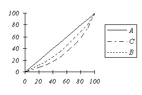
Rice. 5.1. Lorentz curves
Group 1 has 15% of income, Group 2 has 18%, Group 3 has 20%, Group 4 has 22% and Group 5 has 25%.
The fixed asset curve corresponds to an even more uneven distribution of income.
Group 1 gets 10%, Group 2 15%, Group 3 18%, Group 4 20%, Group 5 37%.
The model of income distribution, owned by V. Pareto, is also intended to analyze the nature of income inequality in society. It is constructed as follows:
Let’s denote by Im – the lowest income that a family can receive in a given society. Then, to characterize the relative number of families (in percentage) N (I) receiving an income of not less than I, the ratio can be used:
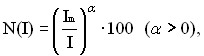
which is a modification of the formula of V. Pareto.
Studies conducted in different countries and at different time periods suggest that this ratio is also applicable when it comes to income from real estate and capital investments. At the same time, the α indicator is usually in the range from 1.2 to 2. Obviously, lower values of α correspond to a more even distribution of income in society, and a high value of α indicates a sharp differentiation of income. In the literature, one can find the opinion that with a α = 1.5, there is a relatively fair distribution of income (Fig. 5.2.).
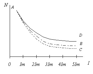
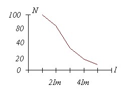
Rice. 5.2. Model of income distribution of V. Pareto
Here, the AV line corresponds to the distribution of income with α = 1.5, the AC and AD lines to the values of α = 2 and α = 1.2.
The division into income groups in the case of α = 1.5 can be performed as follows:
the first group, which has an income from Im to 2Im, consists of 65% of consumers; the second group, has an income from 2Im to 3Im, includes 17% of consumers; the third group with an income of 3Im to 4Im, it includes 7% of consumers, etc. (Fig. 5.3.).
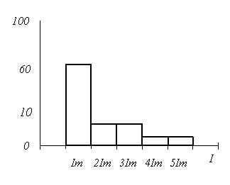
Rice. 5.3. Income groups of the population at α=1.5
The results of studies conducted in societies where the main source of income is wages, show that these incomes are distributed rather along a normal curve, however, not quite symmetrical and with truncated ends (Fig. 5.4.).
This type of curve is explained by the presence of both the lower and upper limits of earnings; moreover, the possibility of obtaining high wages is limited due to the influence of many factors, the combined influence of which leads to a quasi-ormal income distribution curve.
Rice. 5.4. Normal Income Distribution Curve
The division into income groups in this case has the form shown in Fig. 5.5.

Rice. 5.5. Quasi-normal distribution of income
The choice of a specific model of income distribution, and therefore the method of formation of income groups, is determined as a result of the analysis of data on consumer income in the society or region in question.
In the further exposition of the basics of the theory of consumption, we will proceed from the fact that this formation of groups has been made and the set of consumers is represented as a set of m groups with numbers i = 1,…,m.
At the same time, as noted above, it is assumed that the members of the group are sufficiently similar in determining their preferences, and, consequently, the whole group can be considered as a single consumer in the formation of demand for goods and services that appear in the consumer market.