Optimal delivery batches for single-product models
The inventory management model in conditions of deterministic demand is a model where the intensity of the receipt of requirements is assumed to be known and constant over time. As is well known, in practice, demand can almost never be specified with certainty; instead, it should be described in probabilistic terms.
Deterministic models are interesting because they allow you to get acquainted with the methods of analysis used in more complex systems. In addition, the results obtained with the help of these models give qualitatively correct judgments about the behavior of the system, even if the hypothesis of deterministic demand is abandoned.
In Fig.4.1. shows the most common case of formation (OA), expenditure (AC) of the stock, then the possible formation of a deficit (CD) and its satisfaction (DS). At point S, stock formation begins again, so that the OS time period is the duration of the cycle considered.
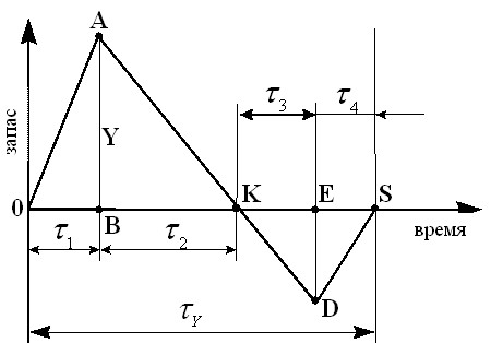
Rice. 4.1. Scheme of inventory movement for deterministic demand.
Thus, in Figure 4.1. shows the scheme of the single-product model, taking into account unmet requirements and the final intensity of consumption and consumption of the stock, where the value of the current stock I is deposited along the ordinate axis, and time t is deposited along the abscissa axis.
Denote:
λ is the intensity of admission;
ν – constant intensity of consumption;
τ1 – duration of stock formation with
velocity λ [reserve units/time units];
τ2 – the time of expenditure of the stock at a rate of ν;
τ3 – the time of formation of a deficit at a rate of ν;
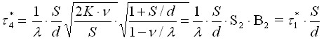
τ4 is the time of repayment of the deficit at a rate of λ.
Then (λ-ν) is the intensity (speed) of replenishment.
The maximum level (volume) of cash stock AB= Y will be:
| (4-1) |
The maximum level of deficit ED=y will be:
| (4-2) |
The duration of the delivery cycle of the next batch or the time of renewal of the ![]()
![]() stock:
stock:
| (4-3) |
Since the demand is satisfied completely, but not always in a timely manner, the size of the delivery![]()
![]() batch:
batch:
| (4-4) |
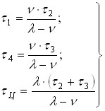
Expressing ![]()
![]() ,
, ![]() and through
and through ![]() and
and ![]()
![]() from (4-1) and (4-2), respectively, we get:
from (4-1) and (4-2), respectively, we get:
| (4-5) |
The total cost of this stockpiling system consists of:
costs ![]()
![]() from the placement of inventories that do not depend on the value
from the placement of inventories that do not depend on the value ![]() ; costs from the maintenance of stocks
; costs from the maintenance of stocks ![]() ; costs from the presence of a deficit
; costs from the presence of a deficit ![]() .
.
Magnitude:
| (4-6) |
where ![]()
![]() are the unit costs of storage and immobilization of funds
are the unit costs of storage and immobilization of funds
[ rub./unit. 60 minutes].
Losses due to the lack of products for which claims are made, or from a deficit, are considered proportional to the average value of the debt requirements and the time of their implementation:
| (4-7) |
where ![]()
![]() are the unit costs of scarcity, i.e. losses associated with the shortage of a unit of output per unit of time.
are the unit costs of scarcity, i.e. losses associated with the shortage of a unit of output per unit of time.
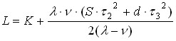
Given the obtained expressions , and , we get a formula for the total costs ![]()
![]() in the system during the cycle
in the system during the cycle ![]() :
:![]()
![]()
![]()
| (4-8) |
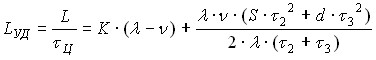
hence the unit cost per cycle will be:
| (4-9) |
Let’s find the optimal values of ?2* and ?3* from the condition that:
| and |
| (4-10) |


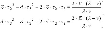
The conditions (4-10) allow us to obtain a system of two equations with two unknowns ![]()
![]() and
and ![]() :
:
| (4-11) |
Let’s denote ![]()
![]() and divide the first of the equations of the system (4-11) by the second, we will find:
and divide the first of the equations of the system (4-11) by the second, we will find:
![]()
![]() .
.
 From , and then
| (4-12) |

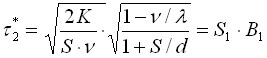
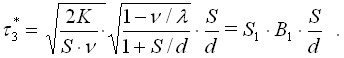
Substituting (4-12) into any of the equations of the system (4-11), we get the optimal values:
| (4-13) |
| (4-14) |
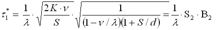
Taking into account (4-13) and (4-14), from (4-5) we get the optimal values of two more components of the duration of the reserve renewal cycle:
| (4-15) |
| (4-16) |
Substituting ?2* and ?2* in the formulas (4-5) and (4-4), we get the optimal values of the repetition cycle of the order and the batch of one-product delivery:
?c*=? 2· K/(S·ν)·? (1+ S / d)/ (1-ν/λ)= S1/B1 (4-17)
q* = ? 2· K·ν/S·? (1+ S / d)/ (1-ν/λ)= S2/B1 (4-18)
Similarly, substituting the values of ?2* and ?3* from (4-13) and (4-14) to (4-9), we determine the optimal unit costs of the system:
Lude*=? 2· K·ν· S? (1-ν/λ)/(1+ S / d)= ? 2· K·ν· S· B1 (4-19)
And, finally, we find the optimal values of the maximum level of cash stock and debt demand:
Y*= ? 2· K·ν/S·? (1-ν/λ)/(1+ S / d)= ? 2· K·ν/(S · B1) (4-20)
y*= S / d·? 2· K·ν/S·? (1-ν/λ)/(1+ S / d)= S / d·? 2· K·ν/(S · B1 ) (4-21)
The total optimal costs of the system during the renewal of the stock will be:
Lobshch *= Lude* ·? c* (4-22)
A model that takes into account unmet requirements at the final intensity of revenues can be widely applied to:
management of the supply of material resources; determining the optimal value of the launch of parts into production, taking into account adjustments on the same technological equipment.
In the second case, K is the costs associated with readjustments. It is assumed that they do not depend on the size of the batch produced and the order of launch of parts into production, λ is the intensity of output (productivity),
?1+ ?4 – time spent on the production of a certain type of product.
From equations (4-13) – (4-22) a number of other partial models can be obtained:
at a high intensity of replenishment, when the entire ordered batch arrives simultaneously; this means that λ>>ν and then ν/λ→0 can be taken. with heavy fines for allowing a deficit of S/d→0, i.e. a deficit is unacceptable (d>>S). when points (a) and (b) operate simultaneously. i.e. ν/λ→0, S/d→0, then we have:
q* = ? 2· K·ν/S
?c*=? 2· K/(S·ν)
Lude*=? 2· K·ν· S
The last model in domestic and foreign literature was called Wilson.
Using the formulas (4-17) – (4-19), it can be shown that due to a reasonable compromise between maintenance costs and losses from the deficit, it is possible to reduce the total cost per unit of time by a factor of 1 + S / d. With ν/λ→0 and high deficit fines, the model in question becomes Wilson’s model.