In general, the coordination of economic interests between participants in a complex process of production, distribution and consumption is most effectively carried out with the help of a market mechanism that acts as a regulator of interrelations between economic entities. In the main version of the market, in conditions of free competition, the producer and the consumer act as independent agents, which allows you to freely make compromise decisions on the conclusion of transactions and develop mutually beneficial conditions for the purchase and sale of certain goods. In a situation where transactions are made by a large number of participants, it can be considered that prices are formed as a result of mass interaction between sellers and buyers, and each individual participant practically does not affect their formation. In this regard, the terms “seller” and “buyer” used below should be understood as a description of aggregated sets of real sellers and buyers, each of whom has its own specific interests. The process of achieving equilibrium itself as An agreed solution is presented as a sequence of actions, each of which can be interpreted either as a real transaction at some intermediate price, or as a negotiating act between the seller and the buyer in order to find out the possible price, volume of supply and demand.
The simplest equilibrium models refer to the case when the subject of transactions is one product, and the participants are an independent seller (producer) and buyer (consumer). Assuming that supply (D) and supply (S) depend only on the price of a commodity (p), say that the equilibrium state in the narrow sense, there is a coincidence of supply and demand
![]()
![]()
where ![]()
![]() is the equilibrium price (Fig. 7.1).
is the equilibrium price (Fig. 7.1).
Equilibrium in the broad sense is any state in which excess demand E(p)= D(p) – S(p) ≤ 0.
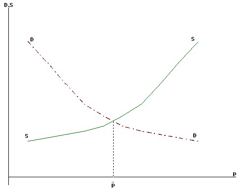
Rice. 7.1. Equilibrium of supply and demand
The actual value of the equilibrium ![]()
![]() price is determined by both the factors of production and consumption.
price is determined by both the factors of production and consumption.
At the same time, on the part of the producer, the price of equilibrium is affected by unit costs for production so that their increase leads to an increase in the equilibrium price, and a decrease leads to its decrease. On the part of the consumer, his income has a significant impact (an increase in income causes an increase in the equilibrium price) and the relative utility of this product for the consumer (its increase also leads to an increase in the equilibrium price).
To illustrate this point, consider the following simple example.
Suppose that the producer of a product strives for maximum profit, provided that the cost function is of the form (see Chapter 4):
![]()
![]()
where c0 is fixed costs,
b is the unit cost ratio.
Then the optimal solution depending on the price (offer function) – has the form:

Let the function of consumer demand then be determined by the relation (see Chapter 3):

where I is the consumer’s income,
γ is the coefficient of relative utility of the product.
The price of equilibrium is defined in this case as the solution of the equation:

Hence:
![]()
![]()
With increasing costs (b), the equilibrium price rises, but the volume of exchange increases
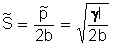
decreases, so that the manufacturer’s cash receipt remains unchanged
![]()
![]()
(it is equal to the share of the consumer’s income that he allocates for the purchase of this product).
As the consumer’s income (I) or relative utility ratio (γ) increases, the equilibrium price also rises, and the volume of exchange also increases.
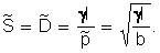
The producer’s cash revenue (and the consumer’s expenses) increases:
![]()
![]()
Thus, the equilibrium price acts as an indicator that combines the diverse interests of the producer and the consumer as a result of a compromise.
The price of equilibrium is usually very sensitive to changes in external conditions or exogenous factors.
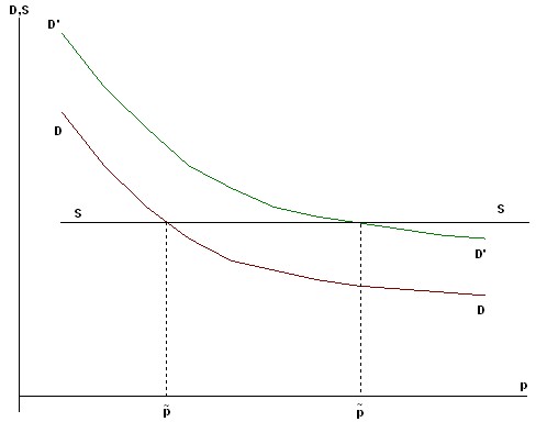
Such factors on the demand side can be changes in the income level of consumers purchasing this product, as well as the influence of fashion and the emergence of new goods for similar purposes. In the case of an increase in income (![]()
![]() ), the demand curve occupies a higher position
), the demand curve occupies a higher position ![]() (Figure 7.2) and the new equilibrium price (
(Figure 7.2) and the new equilibrium price (![]() ) is larger than the previous one (
) is larger than the previous one (![]() ).
).
At the same time, as can be seen, the volume of sales of goods in monetary terms increases (![]()
![]() ).
).
If a more efficient or cheaper substitute for the product we are considering appears on the market, then buyers reduce the share of income that they previously intended for its purchase (![]()
![]() ), and the demand for this product falls. As a result, the demand curve shifts down and to the left (Fig. 7.3) and the new equilibrium price becomes lower than the previous (
), and the demand for this product falls. As a result, the demand curve shifts down and to the left (Fig. 7.3) and the new equilibrium price becomes lower than the previous (![]() ).
).
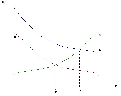
Rice. 7.2. Shifting the demand curve with increasing income
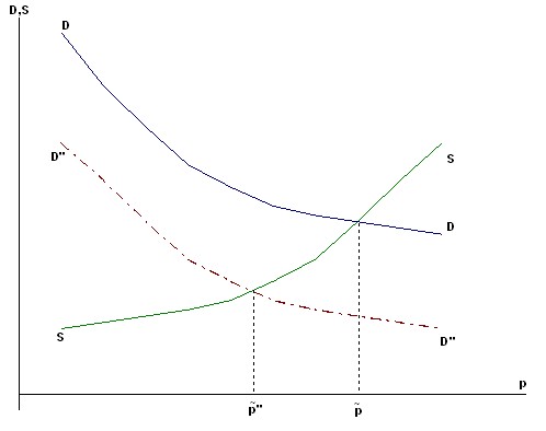
Rice. 7.3. Shifting the demand curve when a cheaper similar product appears on the market
The volume of sales of goods is also decreasing.
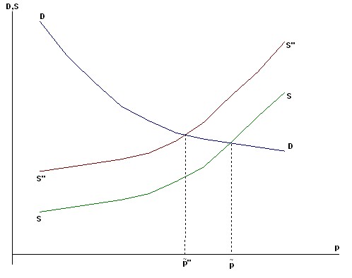
A change in terms on the offer side may also occur due to various circumstances.
For example, a decrease in the level of supply of goods may be caused by a decrease in production due to the severance of pre-existing economic ties; poor harvests of agricultural products; In all these cases, the supply curve is shifted down to the right to the position ![]()
![]() and the new equilibrium price is larger than the old () (
and the new equilibrium price is larger than the old () (![]() Figure 7.4).
Figure 7.4).
Rice. 7.4. A decrease in the volume of supply leads to an increase in the equilibrium price
Note that at the same time the volume of sales in physical terms is decreasing, but in monetary terms it may increase.
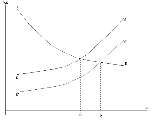
The development of new economical technologies, special state or commercial subsidies can cause the production of goods in the same volumes to be carried out at a lower cost. In this environment, the supply curve shifts left upward (![]()
![]() ) in Figure 7.5 and the equilibrium price decreases (
) in Figure 7.5 and the equilibrium price decreases (![]() ).
).
Rice. 7.5. New technologies, subsidies shift the supply curve upwards, the equilibrium price decreases
A special case is the monopoly market, when the supply is either practically independent of the price (is inelastic), or even decreases as the price increases. In this situation, the change in the equilibrium price is determined by the change in demand (Figure 7.6).
The above analysis allows us to study a more general case, when there is a simultaneous influence of several different factors on the price of equilibrium: for example, consumer incomes increase and additional subsidies or benefits to production are carried out. In such an environment, the opposite tendencies (upwards and downwards in prices) can be mutually repaid and a stable price level is maintained.
Rice. 7.6. In the monopoly market, the offer practically does not depend on the price
If there is an increase in consumer incomes, but production conditions do not improve, then the conditions for uncontrolled price growth, which is usually called demand-pull inflation, appear.
In a situation where consumer incomes practically do not increase, but producers’ costs increase, another type of inflation appears: cost-push inflation. In the real world, the various causes of inflation are intertwined and the classification of inflationary phenomena becomes very difficult.
The quantitative study of changes in the equilibrium position due to variations in external conditions and their corresponding parameters is called comparative statics. Let’s show with examples how such an analysis is carried out.
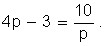
Suppose that the function of offering some product is represented by the formula:
S(p) = 4p – 3,
and the demand function is:
 .
.
The price of equilibrium (![]()
![]() ) is the solution of the equation:
) is the solution of the equation:
Obviously, ![]()
![]() and the volume of sales
and the volume of sales ![]()
I. Suppose first that consumer income has increased by 10%, and now the demand function looks like this:

The new equilibrium price satisfies the equation
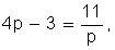
where does the new equilibrium price come from?
![]()
![]()
Thus, we see that a 10% increase in revenue has led to a price increase of almost 4%. This means that the price elasticity of the equilibrium for income is approximately equal to
![]()
![]()
i.e. on average, with an increase in income by 1%, the price will increase by 0.4%.
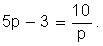
2. In this example, consider the case when the demand function remained the same, but there was a decrease in prices for raw materials and materials that are used in the production of this product, as a result of which the supply function changed (became more elastic). Let it be expressed as follows:
S(p) = 5p – 3.
Now the equilibrium price (![]()
![]() ) is from the equation:
) is from the equation:
Hence we have: ![]()
![]()
Thus, with an increase in the elasticity of supply at the price by 20%, the equilibrium price decreased by 12.7%. It follows that, on average, a decrease in prices for raw materials and materials by 1% results in a decrease in the equilibrium price of goods by 0.6%.
Methods of comparative statics are also used in a more complex situation, when it comes to the equilibrium in the markets of many goods. They provide an opportunity to assess the effectiveness and efficiency of many measures of public administration of the economy.