When modeling consumer demand, the same level of utility of different combinations of consumer goods is graphically displayed using the indifference curve.
In economic and mathematical models of production, each technology can be graphically represented by a point, the coordinates of which reflect the minimum required expenditure of resources K and L for the production of a given volume of output. The set of such points form a line of equal output, or isoquant. Thus, the production function is graphically represented by a family of isoquants. The farther away from the origin of the isoquant, the greater the volume of production it reflects. Unlike the indifference curve, each isoquant characterizes a quantified volume of output. Figure 6.1 shows three isoquants corresponding to a production volume of 200, 300, and 400 units.
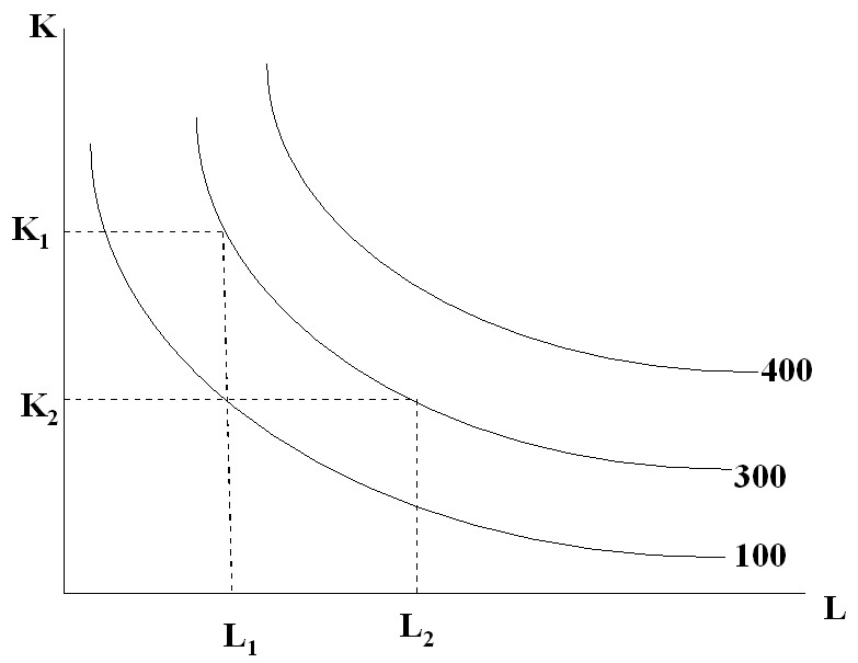
Rice. 6.1. Isoquants corresponding to different production volumes
It can be said that to produce 300 units of output, you need K1 units of capital and L1 units of labor or K2 units of capital or L2 units of labor, or any other combination of them from the set that is represented by the isoquant Y2 = 300.
In general, in the set X of the permissible sets of production factors, a subset of Xc is distinguished, called the isoquant of the production function, is distinguished, which is characterized by the fact that for each vector ![]()
![]() the equality is true:
the equality is true:
f(x) = c
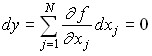
Thus, for all sets of resources corresponding to the isoquant, the volumes of output are equal. Essentially, isoquant is a description of the possibility of mutual substitution of factors in the production process, providing a constant volume of production. In this regard, it is possible to determine the coefficient of mutual substitution of resources using a differential ratio along any isocvent.
 .
.
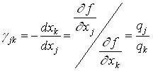
Hence, the coefficient of equivalent replacement of a pair of factors j and k is:
 .
.
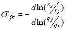
The resulting ratio shows that if production resources are replaced in a ratio equal to the ratio of incremental productivity, then the quantity of output remains unchanged. It must be said that knowledge of the production function allows us to characterize the scale of the possibility of mutual replacement of resources in effective technological methods. To achieve this goal, the coefficient of elasticity of resource substitution by product is used:
 ,
,
which is calculated along the isoquant at the constant level of costs of other production factors. The value σjk is a characteristic of the relative change in the coefficient of mutual substitution of resources with a change in the ratio between them. If the ratio of interchangeable resources changes by σjk percent, then the coefficient of mutual substitution will change by 1 percent. In the case of a linear production function, the coefficient of mutual substitution remains unchanged at any ratio of resources used and therefore it can be considered that elasticity![]()
![]() . Accordingly, large values
. Accordingly, large values ![]() of σjk indicate that greater freedom is possible in replacing production factors along the isocquant and at the same time the main characteristics of the production functions (productivity, interchange coefficient) will change very little.
of σjk indicate that greater freedom is possible in replacing production factors along the isocquant and at the same time the main characteristics of the production functions (productivity, interchange coefficient) will change very little.
For power production functions, the equality σjk=1 is valid for any pair of interchangeable resources. In the practice of forecasting and pre-planned calculations, constant replacement elasticity (CES) functions are often used, having the form:
 .
.
For this function, the resource replacement elasticity coefficient:

and does not change depending on the amount and ratio of resources expended. At small values of σjk, resources can replace each other only in small sizes, and in the limit at σjk = 0 they lose the property of interchangeability and act in the production process only in a constant relation, i.e. they are complementary. An example of a production function that describes production under conditions of using complementary resources is the “output-cost” function, which has the form:
![]()
![]() ,
,
where aj is the constant resource efficiency of j-th of the production factor. It is not difficult to see that a production function of this type determines output by a “bottleneck” on the set of production factors used. Different cases of behavior of isoquant production functions for different values of the substitution elasticity coefficients are presented on the graph (Fig. 6.2).
The representation of the effective technological set using the scalar production function is insufficient in cases where it is impossible to do with a single indicator describing the results of the production facility, but it is necessary to use several (M) output indicators. Under these conditions, the vector production function can be used:
![]()
![]() ,
,

Rice. 6.2. Various Cases of Isoquant Behavior
An important concept of marginal (differential) productivity is introduced by the ratio:
 ,
,
A similar generalization is allowed by all other main characteristics of scalar PF.
Like indifference curves, isocquants are also divided into different types.
For a linear production function of the form:
Y = A + b1K + b2L , where
Y – production volume;
A, b1, b2 – parameters;
K, L – capital expenditure and there,
and the complete replacement of one resource by another isoquant will have a linear form (Figure 6.3).
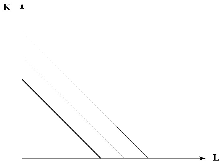
Rice. 6.3. Linear type isoquants
For the power production function, Y = AKαLβ will have the form of curves (Figure 6.4).

Rice. 6.4. Isoquants of the power production function
If the isoquant reflects only one technological method of producing a given product, then labor and capital are combined in the only possible combination (Fig. 6.5).
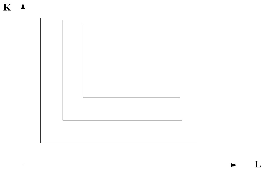
Rice. 6.5. Isoquants with tight complementarity of resources
Such isocquants are sometimes called isocquants of the Leontief type, after the American economist V.V. Leontiev, who put this type of isoquant in the basis of the input-output method developed by him.
Isoquants of this configuration are used in linear programming to substantiate the theory of optimal resource allocation. Broken isocquates most realistically represent the technological capabilities of many production facilities. However, in economic theory, it is traditional to use mainly curves of isocquans, which are obtained from broken ones with an increase in the number of technologies and an increase in the fracture points, respectively.