Suppose it is necessary to find the optimal plan for the production of two types of products (x1 and x2), i.e. such a plan in which the target function (total profit) would be maximum, and the available resources would be used in the best way. The task conditions are shown in the table:
Type of production | Resource consumption rate per unit of output | Profit per unit of product | ||
And | In | With | ||
1 | 2 | 0,1 | 3,5 | 4 |
2 | 1 | 0,5 | 1 | 5 |
Volume | 12 | 4 | 18 |
The optimization model of the problem will be recorded as follows:
(a) Objective function:
![]()
![]()
b) Restrictions:
2×1 + x2 ![]()
![]() 12 (resource limit A);
12 (resource limit A);
0.1×1 + 0.5×2 ![]()
![]() 4 (resource limit B);
4 (resource limit B);
3.5×1 + x2 ![]()
![]() 18 (resource limit C).
18 (resource limit C).
c) the condition of non-negativity of variables:
![]()
![]()
This and similar optimization models can be demonstrated graphically (Fig.3.3.).
Let’s transform our system of constraints by finding x2 in each of the equations, and set them aside on the graph. Any point in this graph with x1 and x2 coordinates represents a variant of the plan to be searched. However, limiting resource A narrows the scope of valid solutions. They can be all points bounded by coordinate axes and a straight line AA, because resource A cannot be consumed more than it is available in the enterprise. If the points are on the straightest line, the resource is fully used.
Similar considerations can be given for resources B and C. As a result, any point lying within the shaded polygon will satisfy the conditions of the problem. This polygon is called the area of valid solutions.
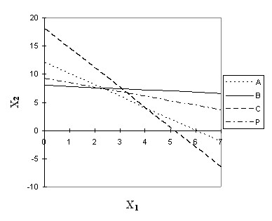
Rice. 3.3. Geometric interpretation of the optimization problem of linear programming
However, we need to find a point at which the maximum of the objective function is reached. To do this, build an arbitrary line 4X1 + 5X2 = 20, as X2 = 4-4 / 5X1 (the number 20 is arbitrary). Let’s denote this line RR. At each point of this line, the profit is the same. Moving this line parallel to its initial position, we will find the point that is most distant from the origin, however, does not go beyond the scope of permissible solutions. This is the M0 point that lies on top of the polygon. The coordinates of this point (![]()
![]() ) will be the desired optimal plan.
) will be the desired optimal plan.